2.1 節練習
練習 2.1
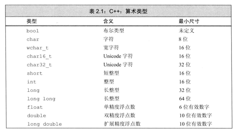
在 C++語言中,int、long、long long 和 short 都屬於整型,區別是 C++標準規定的尺寸的最小值(即該型別在記憶體中所佔的位元數)不同。其中,short是短整型,佔 16 位;int 是整型,佔 16 位;long 和 long long 均為長整型,分別佔 32 位和 64 位。C++標準允許不同的編譯器賦予這些型別更大的尺寸。某一型別佔的位元數不同,它所能表示的資料範圍也不一樣。
大多數整型都可以劃分為無符號型別和帶符號型別,在無符號型別中所有位元
都用來儲存數值,但是僅能表示大於等於 0 的值;帶符號型別則可以表示正數、負數或 0。
float 和 double 分別是單精度浮點數和雙精度浮點數,區別主要是在記憶體中所佔的位元數不同,以及預設規定的有效位數不同。
練習 2.2
在實際應用中,利率、本金和付款既有可能是整數,也有可能是普通的實數。
因此應該選擇一種浮點型別來表示。在三種可供選擇的浮點型別 float、double和 long double 中,double 和 float 的計算代價比較接近且表示範圍更廣,long double 的計算代價則相對較大,一般情況下沒有選擇的必要。綜合以上分析,選擇double 是比較恰當的。
練習 2.3
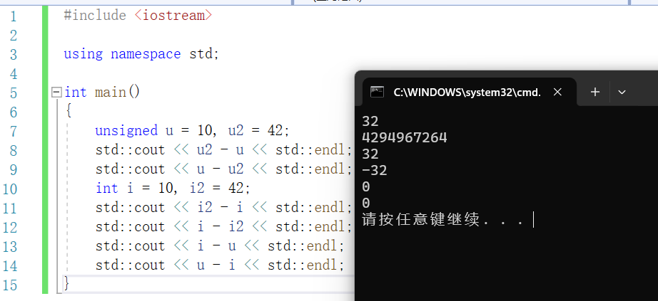
u 和 u2 都是無符號整數,因此 u2-u 得到了正確的結果(42−10=32);
u-u2 也能正確計算,但是因為直接計算的結果是-32,所以在表示為無符號整數時自動加上了模,在此編譯環境中 int 佔 32 位,因此加模的結果是 4294967264。
i 和 i2 都是帶符號整數,因此中間兩個式子的結果比較直觀,42-10=32,
10-42=−32。
在最後兩個式子中,u 和 i 分別是無符號整數和帶符號整數,計算時編譯器先把帶符號數轉換為無符號數,幸運的是,i 本身是一個正數,因此轉換後不會出現異常情況,兩個式子的計算結果都是 0。
不過需要注意的是,一般情況下請不要在同一個表示式中混合使用無符號型別和帶符號型別。因為計算前帶符號型別會自動轉換成無符號型別,當帶符
號型別取值為負時就會出現異常結果。
練習 2.4
見練習 2.3。
練習 2.5
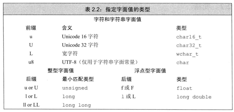
(a) 'a'表示字元 a,L'a'表示寬字元型字面值 a 且型別是 wchar_t,"a"表示字串 a,L"a"表示寬字元型字串 a。
(b) 10 是一個普通的整數型別字面值,10u 表示一個無符號數,10L 表示一個長整型數,10uL 表示一個無符號長整型數,012 是一個八進位制數(對應的十進位制數是 10),0xC 是一個十六進位制數(對應的十進位制數是 12)。
(c) 3.14 是一個普通的浮點型別字面值,3.14f 表示一個 float 型別的單精度浮點數,3.14L 表示一個 long double 型別的擴充套件精度浮點數。
(d) 10 是一個整數,10u 是一個無符號整數,10.是一個浮點數,10e-2 是一個科學計數法表示的浮點數,大小為 10*10^-2=0.1。
附上書上的兩張圖
練習 2.6
第一組定義是正確的,定義了兩個十進位制數 9 和 7。
第二組定義是錯誤的,編譯時將報錯。因為以 0 開頭的數是八進位制數,而數字 9顯然超出了八進位制數能表示的範圍,所以第二組定義無法被編譯透過。
練習 2.7
(a)是一個字串,包含兩個跳脫字元,其中\145 表示字元 e,\012 表示一個換行符,因此該字串的輸出結果是 Who goes with Fergus?
結合書上的原話去理解會更好:
-
我們也可以使用泛化的轉義序列,其形式是\x後緊跟1個或多個十六進位制數字,或者\後緊跟1個、2個或3個八進位制數字,其中數字部分表示的是字元對應的數值。
-
注意,如果反斜線\後面跟著的八進位制數字超過3個,只有前3個數字與\構成轉義序列。例如,"\1234"表示2個字元,即八進位制數123對應的字元以及字元4。相反,\x要用到後面跟著的所有數字,例如,"\x1234"表示一個16位的字元,該字元由這4個十六進位制數所對應的位元唯一確定。因為大多數機器的char型資料佔8位,所以上面這個例子可能會報錯。一般來說,超過8位的十六進位制字元都是與表22中某個字首作為開頭的擴充套件字符集一起使用的。
(b)是一個科學計數法表示的擴充套件精度浮點數,大小為 3.14*10L=31.4。
(c)試圖表示一個單精度浮點數,但是該形式在某些編譯器中將報錯,因為字尾 f 直接跟在了整數 1024 後面;改寫成 1024.f 就可以了。
(d)是一個擴充套件精度浮點數,型別是 long double,大小為 3.14。
練習 2.8
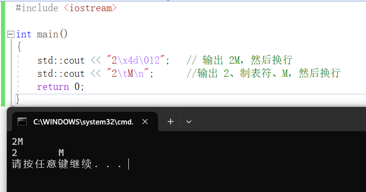
其中,字串"2\x4d\012"先輸出字元 2,緊接著利用跳脫字元\x4d 輸出字
符 M,最後利用跳脫字元\012 轉到新一行。
字串"2\tM\n"先輸出字元 2,然後利用跳脫字元\t 輸出一個製表符,接著輸出字元 M(大寫字母A的ASCII碼是65,小寫字母的a的ASCII碼是97),最後利用跳脫字元\n 轉到新一行。
可以發現,輸出同一個字元有多種方式可供選擇。例如,可以直接輸出字
符 M,也可以透過跳脫字元\x4d 輸出字元 M;可以用跳脫字元\012 換行,也可以用跳脫字元\n 換行。
2.2 節練習
練習 2.9
(a)是錯誤的,輸入運算子的右側需要一個明確的變數名稱,而非定義變數的語句,
改正後的結果是:
int input_value;
std::cin >> input_value;
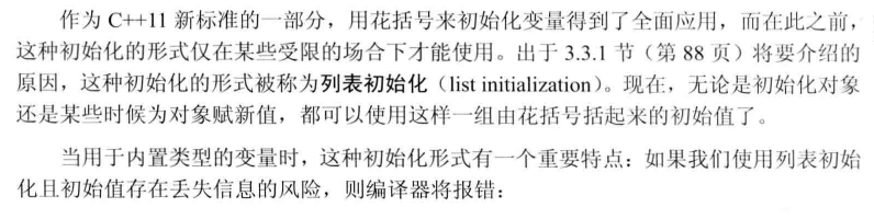
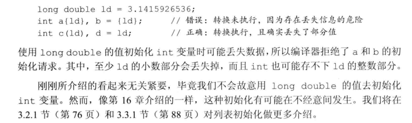
(b)是錯誤的,該語句定義了一個整型變數 i,但是試圖透過列表初始化的方式把浮點數3.14賦值給i,這樣做將造成小數部分丟失,是一種不被建議的窄化操作。
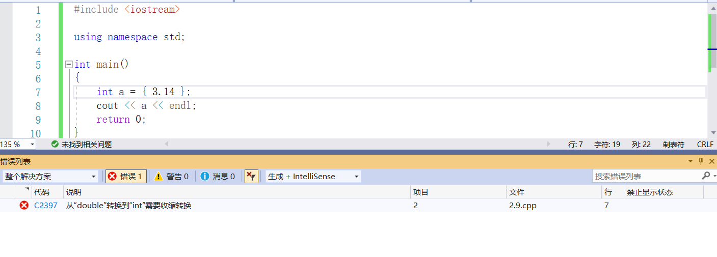
附上書上的原話:
(c)是錯誤的,該語句試圖將 9999.99 分別賦值給 salary 和 wage,但是在宣告語句中宣告多個變數時需要用逗號將變數名隔開,而不能直接用賦值運算子連線,
改正後的結果是:
double salary, wage;
salary = wage = 9999.99;
(d)引發警告,該語句定義了一個整型變數 i,但是試圖把浮點數 3.14 賦值給i,這樣做將造成小數部分丟失,與(b)一樣是不被建議的窄化操作。
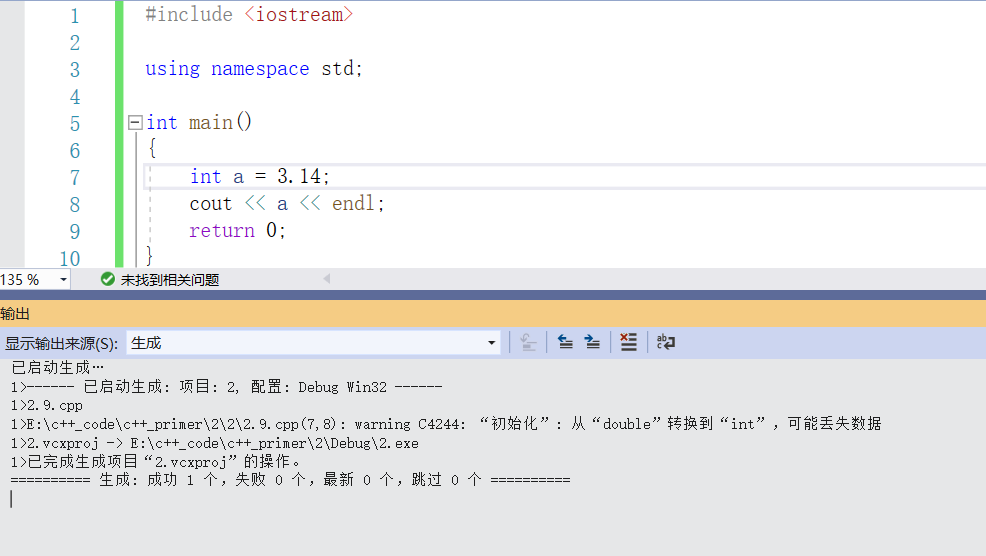
確實引發了一個警告
練習 2.10
對於 string 型別的變數來說,因為 string 型別本身接受無引數的初始化方式,所以不論變數定義在函式內還是函式外都被預設初始化為空串。
對於內建型別 int 來說,變數 global_int 定義在所有函式體之外,根據 C++的規定,global_int 預設初始化為 0;而變數 local_int 定義在 main 函式的內部,將不被初始化,如果程式試圖複製或輸出未初始化的變數,將遇到一個未定義的奇異值。
練習 2.11
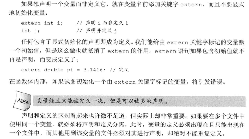
宣告與定義的關係是:宣告使得名字為程式所知,而定義負責建立與名字關聯
的實體。(a)定義了變數 ix,(b)宣告並定義了變數 iy,(c)宣告瞭變數iz。
書上原話:
練習 2.12
(a)是非法的,因為 double 是 C++關鍵字,代表一種資料型別,不能作為變數的名字。
(c)是非法的,在識別符號中只能出現字母、數字和下畫線,不能出現符號-,如果改成“int catch_22;”就是合法的了。
(d)是非法的,因為識別符號必須以字母或下畫線開頭,不能以數字開頭。
(b)和(e)是合法的命名。
練習 2.13
j 的值是 100。C++允許內層作用域重新定義外層作用域中已有的名字,在本題中,int i=42;位於外層作用域,但是變數 i 在內層作用域被重新定義了,因此真正賦予 j 的值是定義在內層作用域中的 i 的值,即 100。
練習 2.14
該程式是合法的,輸出結果是 100 45。
該程式存在巢狀的作用域,其中 for 迴圈之外是外層作用域,for 迴圈內部是內層作用域。首先在外層作用域中定義了 i 和 sum,但是在 for 迴圈內部 i 被重新定義了,因此 for 迴圈實際上是從 i=0 迴圈到了 i=9,內層作用域中沒有重新定義sum,因此 sum 的初始值是 0 並在此基礎上依次累加。最後一句輸出語句位於外層作用域中,此時在 for 迴圈內部重新定義的 i 已經失效,因此實際輸出的仍然是外層作用域的 i,值為 100;而 sum 經由迴圈累加,值變為了 45。
2.3 節練習
練習 2.15
(b)是非法的,引用必須指向一個實際存在的物件而非字面值常量。
(d)是非法的,因為我們無法令引用重新繫結到另外一個物件,所以引用必須初始化。
(a)和(c)是合法的。
練習 2.16
(a)是合法的,為引用賦值實際上是把值賦給了與引用繫結的物件,在這裡是把3.14159 賦給了變數 d。
(b)是合法的,以引用作為初始值實際上是以引用繫結的物件作為初始值,在這裡是把 i 的值賦給了變數 d。
(c)是合法的,把 d 的值賦給了變數 i,因為 d 是雙精度浮點數而 i 是整數,所以該語句實際上執行了窄化操作。
(d)是合法的,把 d 的值賦給了變數 i,與上一條語句一樣執行了窄化操作。
練習 2.17
程式的輸出結果是 10 10。
引用不是物件,它只是為已經存在的物件起了另外一個名字,因此 ri 實際上是i 的別名。在上述程式中,首先將 i 賦值為 5,然後把這個值更新為 10。因為 ri是 i 的引用,所以它們的輸出結果是一樣的。
練習 2.18
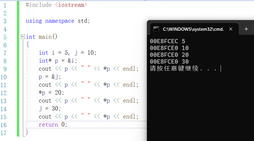
在上述示例中,首先定義了兩個整型變數 i 和 j 以及一個整型指標 p,初始情況下令指標 p 指向變數 i,此時分別輸出 p 的值(即 p 所指物件的記憶體地址)以及 p 所指物件的值,得到 00E8FCEC 和 5。
隨後依次更改指標的值以及指標所指物件的值。p=&j;更改了指標的值,令指
針p指向另外一個整數物件j。*p=20;和j=30是兩種更改指標所指物件值的方式,前者顯式地更改指標 p 所指的內容,後者則透過更改變數 j 的值實現同樣的目的。
練習 2.19
指標“指向”記憶體中的某個物件,而引用“繫結到”記憶體中的某個物件,它們
都實現了對其他物件的間接訪問,二者的區別主要有兩方面:
第一,指標本身就是一個物件,允許對指標賦值和複製,而且在指標的生命周
期內它可以指向幾個不同的物件;引用不是一個物件,無法令引用重新繫結到另外一個物件。
第二,指標無須在定義時賦初值,和其他內建型別一樣,在塊作用域內定義的
指標如果沒有被初始化,也將擁有一個不確定的值;引用則必須在定義時賦初值。
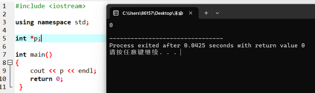
補充:
如果指標被定義為全域性變數,那麼它的初始值為 0
練習 2.20
這段程式碼首先定義了一個整型變數 i 並設其初值為 42;接著定義了一個整型指標 pl,令其指向變數 i;最後取出 pl 所指的當前值,計算平方後重新賦給 pl 所指的變數 i。
第二行的表示宣告一個指標,第三行的表示解引用運算,即取出指標 pl 所指物件的值。
練習 2.21
(a)是非法的,dp 是一個 double 指標,而 i 是一個 int 變數,型別不匹配。
(b)是非法的,不能直接把 int 變數賦給 int 指標,正確的做法是透過取地址運算&i 得到變數 i 在記憶體中的地址,然後再將該地址賦給指標。
(c)是合法的。
練習 2.22
指標 p 作為 if 語句的條件時,實際檢驗的是指標本身的值,即指標所指的地址值。如果指標指向一個真實存在的變數,則其值必不為 0,此時條件為真;如果指標沒有指向任何物件或者是無效指標,則對 p 的使用將引發不可預計的結果。
解引用運算子*p 作為 if 語句的條件時,實際檢驗的是指標所指的物件內容,在上面的示例中是指標 p 所指的 int 值。如果該 int 值為 0,則條件為假;否則,如果該 int 值不為 0,對應條件為真。
練習 2.23
在 C++程式中,應該儘量初始化所有指標,並且儘可能等定義了物件之後再定義指向它的指標。如果實在不清楚指標應該指向何處,就把它初始化為 nullptr 或者 0,這樣程式就能檢測並知道它有沒有指向一個具體的物件了。
其中,nullptr是 C++11 新標準剛剛引入的一個特殊字面值,它可以轉換成任意其他的指標型別。在此前提下,判斷 p 是否指向合法的物件,只需把 p 作為 if 語句的條件即可,如果p 的值是 nullptr,則條件為假;反之,條件為真。
如果不注意初始化所有指標而貿然判斷指標的值,則有可能引發不可預知的結
果。一種處理的辦法是把 if(p)置於 try 結構中,當程式塊順利執行時,表示 p 指向了合法的物件;當程式塊出錯跳轉到 catch 語句時,表示 p 沒有指向合法的物件。
練習 2.24
p 是合法的,因為 void*是一種特殊的指標型別,可用於存放任意物件的地址。
lp 是非法的,因為 lp 是一個長整型指標,而 i 只是一個普通整型數,二者的型別不匹配。
練習 2.25
(a)ip 是一個整型指標,指向一個整型數,它的值是所指整型數在記憶體中的地址;i是一個整型數;r 是一個引用,它繫結了 i,可以看作是 i 的別名,r 的值就是 i 的值。
(b)i 是一個整型數;ip 是一個整型指標,但是它不指向任何具體的物件,它的值被初始化為 0。
(c)ip是一個整型指標,指向一個整型數,它的值是所指整型數在記憶體中的地址;ip2 是一個整型數。
2.4 節練習
練習 2.26
本題的所有語句應該被看作是順序執行的,即形如:
const int buf;
int cnt = 0;
const int sz = cnt;
++cnt;
++sz;
(a)是非法的,const 物件一旦建立後其值就不能改變,所以 const 物件必須初始化。該句應修改為 const int buf = 10。
(b)和(c)是合法的。
(d)是非法的,sz 是一個 const 物件,其值不能被改變,當然不能執行自增操作。
練習 2.27
(a)是非法的,非常量引用 r 不能引用字面值常量 0。
(b)是合法的,p2 是一個常量指標,p2 的值永不改變,即 p2 永遠指向變數 i2。
(c)是合法的,i 是一個常量,r 是一個常量引用,此時 r 可以繫結到字面值常量 0。
(d)是合法的,p3 是一個常量指標,p3 的值永不改變,即 p3 永遠指向變數 i2;同時 p3 指向的是常量,即我們不能透過 p3 改變所指物件的值。
(e)是合法的,p1 指向一個常量,即我們不能透過 p1 改變所指物件的值。
(f)是非法的,引用本身不是物件,因此不能讓引用恆定不變。
(g)是合法的,i2 是一個常量,r 是一個常量引用。
練習 2.28
(a)是非法的,cp 是一個常量指標,因其值不能被改變,所以必須初始化。
(b)是非法的,cp2 是一個常量指標,因其值不能被改變,所以必須初始化。
(c)是非法的,ic 是一個常量,因其值不能被改變,所以必須初始化。
(d)是非法的,p3 是一個常量指標,因其值不能被改變,所以必須初始化;同時p3 指向的是常量,即我們不能透過 p3 改變所指物件的值。
(e)是合法的,但是 p 沒有指向任何實際的物件。
練習 2.29
(a)是合法的,常量 ic 的值賦給了非常量 i。
(b)是非法的,普通指標 p1 指向了一個常量,從語法上說,p1 的值可以隨意改變,顯然是不合理的。
(c)是非法的,普通指標 p1 指向了一個常量,錯誤情況與上一條類似。
(d)是非法的,p3 是一個常量指標,不能被賦值。
(e)是非法的,p2 是一個常量指標,不能被賦值。
(f)是非法的,ic 是一個常量,不能被賦值。
練習 2.30
v2 是頂層 const,表示一個整型常量;p2 和r2 是底層 const,分別表示它們所指(所引用)的物件是常量。
p3 既是頂層const又是底層const,p3 是一個常量指標,指向一個整形常量。
練習 2.31
在執行複製操作時,頂層 const 和底層 const 區別明顯。其中,頂層 const不受影響,這是因為複製操作並不會改變被複製物件的值。底層 const 的限制則不容忽視,拷入和拷出的物件必須具有相同的底層 const 資格,或者兩個物件的資料型別必須能夠轉換。一般來說,非常量可以轉換成常量,反之則不行。
r1=v2;是合法的,r1 是一個非常量引用,v2 是一個常量(頂層 const),把 v2的值複製給 r1 不會對 v2 有任何影響。
p1=p2;是非法的,p1 是普通指標,指向的物件可以是任意值,p2 是指向常量的指標(底層 const),令 p1 指向 p2 所指的內容,有可能錯誤地改變常量的值。
p2=p1;是合法的,與上一條語句相反,p2 可以指向一個非常量,只不過我們
不會透過 p2 更改它所指的值。
p1=p3;是非法的,p3 包含底層 const 定義(p3 所指的物件是常量),不能把p3 的值賦給普通指標。
p2=p3;是合法的,p2 和 p3 包含相同的底層 const,p3 的頂層 const 則可以忽略不計。
練習 2.32
上述程式碼是非法的,null 是一個 int 變數,p 是一個 int 指標,二者不能直接繫結。僅從語法角度來說,可以將程式碼修改為:
int null = 0, *p = &null;
顯然,這種改法與程式碼的原意不一定相符。另一種改法是使用 nullptr:
int null = 0, *p = nullptr;
2.5 節練習
練習 2.33
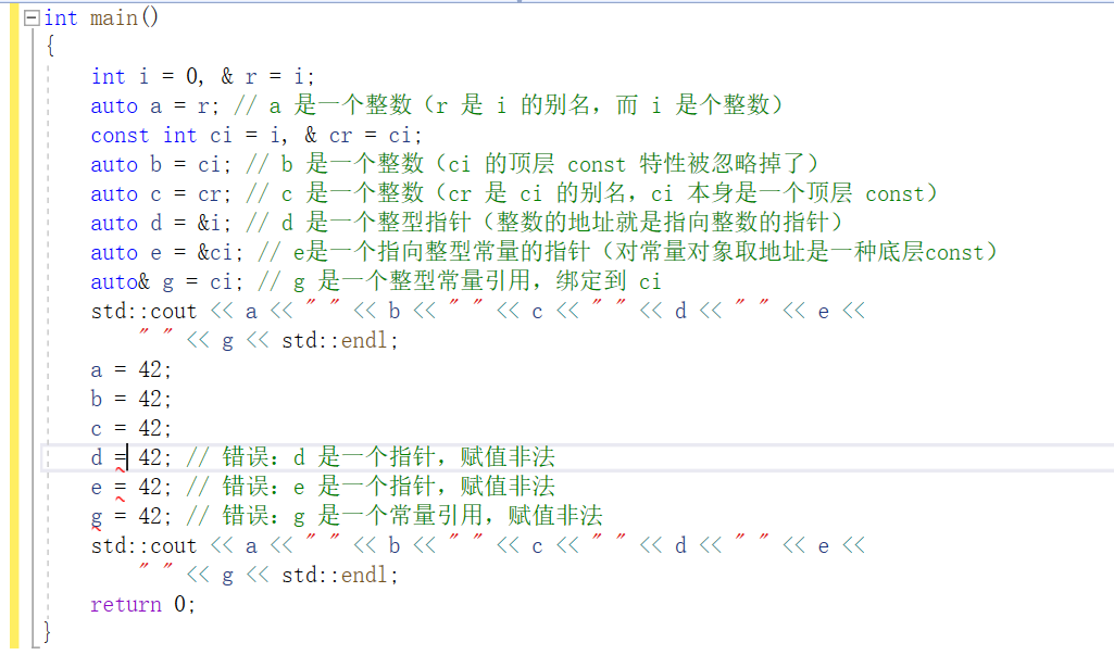
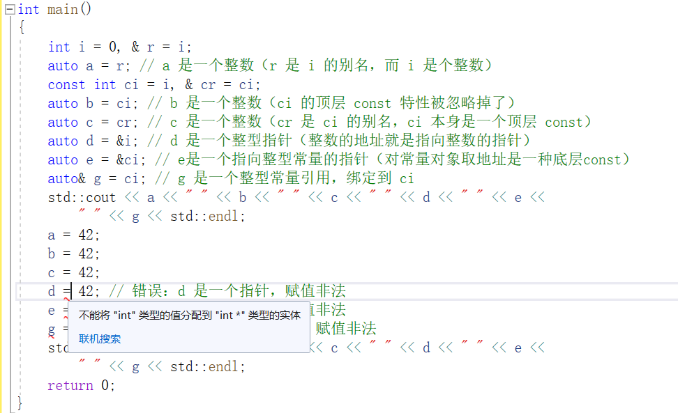
前 3 條賦值語句是合法的,原因如下:
r 是 i 的別名,而 i 是一個整數,所以 a 的型別推斷結果是一個整數;
ci 是一個整型常量,在型別推斷時頂層 const 被忽略掉了,所以 b 是一個整數;
cr 是 ci的別名,而 ci 是一個整型常量,所以 c 的型別推斷結果是一個整數。
因為 a、b、c都是整數,所以為其賦值 42 是合法的。
後 3 條賦值語句是非法的,原因如下:
i 是一個整數,&i 是 i 的地址,所以 d 的型別推斷結果是一個整型指標;
ci是一個整型常量,&ci 是一個整型常量的地址,所以 e 的型別推斷結果是一個指向整型常量的指標;
ci 是一個整型常量,所以 g 的型別推斷結果是一個整型常量引用。
因為 d 和 e 都是指標,所以不能直接用字面值常量為其賦值;g 繫結到了整型常量,所以不能修改它的值。
練習 2.34
Visual Studio居然自己就把下面的d,e,g的錯誤報出來了,而且還有解釋
比如:
練習 2.35
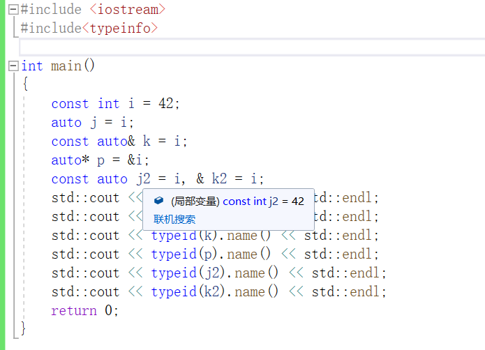
i 是一個整型常量,
j 的型別推斷結果是整數,
k 的型別推斷結果是整型常量
p 的型別推斷結果是指向整型常量的指標
j2 的型別推斷結果是整形常量,
k2 的型別推斷結果是整形常量引用。

這個程式的輸出的型別不太全面,有些沒有把const輸出出來。
可以透過把滑鼠放到對應變數上檢視該變數型別。
練習 2.36
在本題的程式中,初始情況下 a 的值是 3、b 的值是 4。
decltype(a) c=a;使用的是一個不加括號的變數,因此 c 的型別就是 a 的型別,即該語句等同於 int c=a;,此時 c 是一個新整型變數,值為 3。
decltype((b)) d=a;使用的是一個加了括號的變數,因此 d 的型別是引用,即該語句等同於 int &d=a;,此時 d 是變數 a 的別名。
執行++c; ++d;時,變數 c 的值自增為 4,因為 d 是 a 的別名,所以 d 自增 1意味著 a 的值變成了 4。
當程式結束時,a、b、c、d 的值都是 4。
附上書上原話:
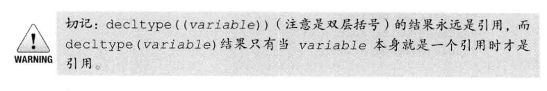
練習 2.37
根據 decltype 的上述性質可知,c 的型別是 int,值為 3;
表示式 a=b 作為decltype 的引數,編譯器分析表示式並得到它的型別作為 d 的推斷型別,但是不實際計算該表示式,所以 a 的值不發生改變,仍然是 3;
d 的型別是 int&,d 是 a的別名,值是 3;
b 的值一直沒有發生改變,為 4。
練習 2.38
auto 和 decltype 的區別主要有三個方面:
-
第一,auto型別說明符用編譯器計算變數的初始值來推斷其型別,而decltype雖然也讓編譯器分析表示式並得到它的型別,但是不實際計算表示式的值。
-
第二,編譯器推斷出來的 auto 型別有時候和初始值的型別並不完全一樣,編譯器會適當地改變結果型別使其更符合初始化規則。例如,auto 一般會忽略掉頂層const,而把底層const保留下來。與之相反,decltype會保留變數的頂層const。
-
第三,與 auto 不同,decltype 的結果型別與表示式形式密切相關,如果變數名加上了一對括號,則得到的型別與不加括號時會有不同。如果 decltype 使用的是一個不加括號的變數,則得到的結果就是該變數的型別;如果給變數加上了一層或多層括號,則編譯器將推斷得到引用型別。
舉個例子來說明:
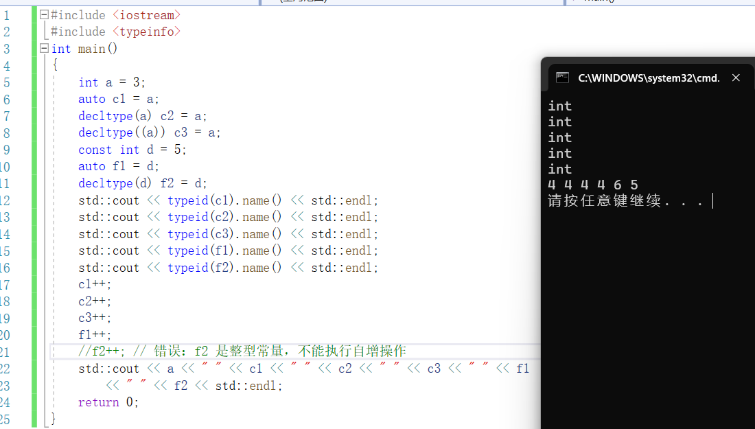
對於第一組型別推斷來說,a 是一個非常量整數,c1 的推斷結果是整數,c2 的推斷結果也是整數,c3 的推斷結果由於變數 a 額外加了一對括號所以是整數引用。
c1、c2、c3 依次執行自增操作,因為 c3 是變數 a 的別名,所以 c3 自增等同於 a自增,最終 a、c1、c2、c3 的值都變為 4。
對於第二組型別推斷來說,d 是一個常量整數,含有頂層 const,使用 auto推斷型別自動忽略掉頂層 const,因此 f1 的推斷結果是整數;decltype 則保留頂層 const,所以 f2 的推斷結果是整數常量。f1 可以正常執行自增操作,而常量f2 的值不能被改變,所以無法自增。
2.6 節練習
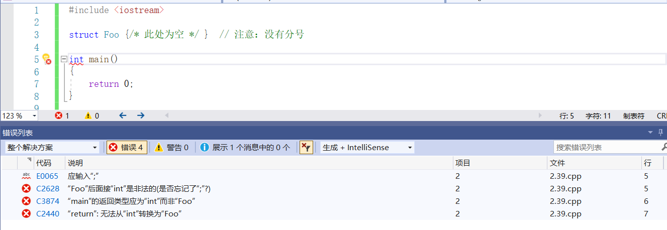
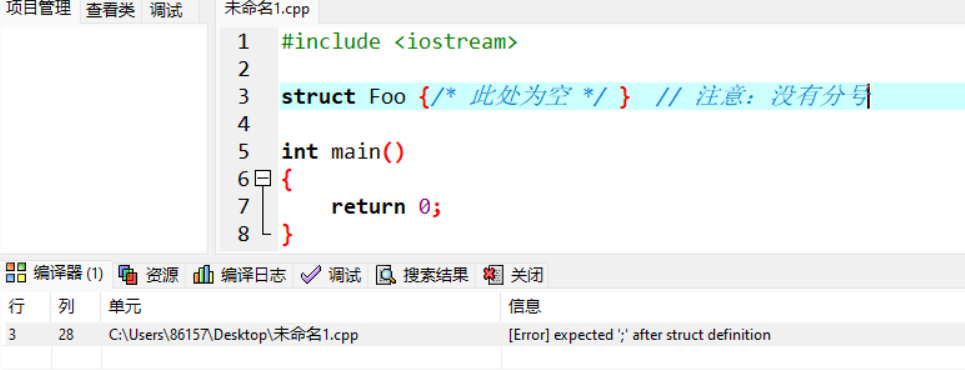
練習 2.39
該程式無法編譯透過,原因是缺少了一個分號。因為類體後面可以緊跟變數名
以示對該型別物件的定義,所以在類體右側表示結束的花括號之後必須寫一個分號。
稍作修改,該程式就可以編譯透過了。
struct Foo { /* 此處為空 */ };
int main ()
{
 return 0;
}
嘗試了下,報錯情況如下:
在Visual Studio中:
在Dev-C++中:
練習 2.40
原書中的程式包含 3 個資料成員,分別是 bookNo(書籍編號)、units_sold(銷售量)、revenue(銷售收入),
新設計的 Sales_data 類細化了銷售收入的計算方式,在保留 bookNo 和 units_sold 的基礎上,新增了sellingprice(零售價、原價)、saleprice(實售價、折扣價)、discount(折扣),其中discount=saleprice/sellingprice。
struct Sales_data {
 std::string bookNo; // 書籍編號
 unsigned units_sold = 0; // 銷售量
 double sellingprice = 0.0; // 零售價
 double saleprice = 0.0; // 實售價
 double discount = 0.0 // 折扣
};
練習 2.41
不太確定
練習 2.42
不太確定