
本文是一個基於 NebulaGraph 圖演演算法、圖資料庫、機器學習、GNN 的 Fraud Detection 方法綜述。在閱讀本文了解欺詐檢測的基本實現方法之餘,也可以在我給大家準備的 Playground 上跑下資料。
下面進入本次圖資料庫的欺詐檢測實踐:
建立反欺詐圖譜
欺詐檢測實踐的第一步,是面向關聯關係對現有的歷史資料、標註資訊進行屬性圖建模。一般來說,這種原始資料是由多個表結構中的銀行、電子商務或者保險行業裡的交易事件記錄、使用者資料和風控標註組成,而建模過程就是抽象出我們關心的實體、實體間的關聯關係及其中有意義的屬性。
一般來說,自然人、公司實體、電話號碼、地址、裝置(比如終端裝置、網路地址、終端裝置所連線的 Wi-Fi SSID 等)、訂單都是實體。其他資訊,比如:風險標註(是否高風險、風險描述等)、自然人和公司實體的資訊(職業、收入、學歷等)都作為實體的屬性來建模。
下圖是一個貸款反欺詐的示例建模,你可以訪問 https://github.com/wey-gu/fraud-detection-datagen 獲取這份資料生成器程式碼和示例資料。

圖資料庫查詢識別風險
有了一張囊括了人、公司、歷史貸款申請記錄、電話、線上申請的網路裝置的圖譜,我們可以挖掘一些有意思的資訊。
事實上,很多被發現且被有效阻止,避免損失的騙保行為都是具有群體聚集性的。比如:欺詐團夥可能是一小批人(比如:3 到 5 人)有組織地收集更大規模的身份證資訊(比如:30 張),同時申請多個金融機構的大量貸款。在放款後,團夥丟棄這批留下了違約記錄的身份證,再選擇下一批身份證如法炮製。
這種團夥作案的方式因為利用了大量新的身份資訊,完全利用歷史記錄中的黑名單去規避風險的方式是無效的。不過,從關聯關係的角度出發,這些模式是一定程度上可以被及時識別出來的。
這些可以被識別出的欺詐行為,我把它分成兩種:
一種是風控專家可以直接用某種模式來描述的,例如:和已經被標註為高風險的實體有直接或者間接的關聯關係,像是新訂單申請人使用了和過往高風險記錄相同的網路裝置。這種模式對應到圖譜中,透過一個圖查詢就可以實時給出結果。
另一種是隱含在資料的關聯關係背後,需要透過圖演演算法挖掘得出的風險提示,例如:給定的實體與有限的標註高風險實體沒有匹配的關聯,但是它在圖中形成了聚集性。這就提示我們,這可能是一個尚未得手、進行中的團夥貸款詐騙貸款申請。這種情況下,可以透過定期在歷史資料中批次執行社群發現演演算法得出,並在高聚集社群中利用中心性演演算法給出核心實體,一併提示給風險專家進行後續評估和風險標註。
基於圖譜與專家圖模式匹配的欺詐檢測示例
在開始之前,我們利用 Nebula-UP 來一鍵部署一套 NebulaGraph 圖資料庫:
curl -fsSL nebula-up.siwei.io/install.sh | bash首先,我們把前面建模的圖譜載入到 NebulaGraph 裡:
# 克隆資料集程式碼倉庫
git clone https://github.com/wey-gu/fraud-detection-datagen.git
cp -r data_sample_numerical_vertex_id data
# 去掉表頭
sed -i '1d' data/*.csv
docker run --rm -ti \
    --network=nebula-net \
    -v ${PWD}:/root/ \
    -v ${PWD}/data/:/data \
    vesoft/nebula-importer:v3.1.0 \
    --config /root/nebula_graph_importer.yaml
有了這樣一個圖譜,風控專家可以在視覺化探索工具 NebulaGraph Studio 中按需探索實體之間的關係,繪製相應的風險模式:

如上所示,我們可以明顯看到一個群控裝置的風險模式,這個模式可以被交給圖資料庫開發者,抽象成可以被風控應用定期、實時查詢的語句:
## 針對一筆交易申請關聯查詢
MATCH (n) WHERE id(n) == "200000010265"
OPTIONAL MATCH p_shared_d=(n)-[:used_device]->(d)<-[:used_device]-(:applicant)-[:with_phone_num]->(pn:phone_num)<-[e:with_phone_num]-(:applicant)
RETURN p_shared_d
我們可以很容易在此模型之上,透過修改返回的關聯裝置計數,作為意向指標查詢的判斷 API:
## 群控指標
MATCH (n) WHERE id(n) == "200000010265"
OPTIONAL MATCH p_shared_d=(n)-[:used_device]->(d)<-[:used_device]-(:applicant)-[:with_phone_num]->(pn:phone_num)<-[e:with_phone_num]-(:applicant)
RETURN count(e)
基於此,我們利用有限的標註資料和專家資源,可以建立一個相對有效的風控系統,去更高效地控制團夥欺詐作案風險。
另一個利用標註風險節點的查詢是找到相關聯節點高風險屬性的數量:
MATCH p_=(p:applicant)-[*1..2]-(p2:applicant) WHERE id(p)=="200000014810" AND p2.applicant.is_risky == "True" RETURN p_ LIMIT 100可以從這個路徑查詢看到 200000014810 相連線的申請人中有不少是高風險的(也能看出聚集的裝置們)。

因此,我們可以定義相連高風險點數量為一個指標:
MATCH (p:applicant)-[*1..2]-(p2:applicant) WHERE id(p)=="200000014810" AND p2.applicant.is_risky == "True" RETURN count(p2)然而,在現實應用中,大多數的標註資料的獲取還是過於昂貴,那麼有沒有什麼方法是更有效利用有限的風險標註和圖結構來預測出風險的呢?
答案是肯定的。
利用圖擴充標註
Xiaojin Z. 和 Zoubin G. 在論文:Learning from Labeled and Unlabeled Data with Label Propagation(CMU-CALD-02-107)中,利用標籤傳播 Label Propagation 演演算法把有限的標註資訊在圖上透過關聯關係傳播到更多實體中。
在標籤傳播演演算法的加持下,我們建立的圖譜可以很容易地藉助有限的高風險標註,去“傳播”產生更多的標註資訊。這些擴充套件出來的標註資訊一方面可以在實時的圖查詢中給出更多的結果,另一方面,它還能作為風控專家重要的輸入資訊,幫助推進反欺詐調查行動的開展。
一般來說,我們可以透過定期離線地全圖掃描資料,再用圖演演算法擴充、更新標註,最後將有效的更新標註寫回到圖譜之中。
類似的方法還有 SinDiffusion,感興趣的同學可以去了解一下。
圖演演算法擴充欺詐風險標註
下面,我給出一個可以跑通的示例。在這個例子中,我用到了經典詐騙識別資料集 Yelp。這份資料不只會用在這個例子中,後邊 GNN 方法中的示例也會用到,所以大家可以放心把資料匯入 NebulaGraph。
資料生成匯入的方法在這裡:https://github.com/wey-gu/nebulagraph-yelp-frauddetection
cd ~
git clone https://github.com/wey-gu/nebulagraph-yelp-frauddetection
cd nebulagraph-yelp-frauddetection
python3 -m pip install -r requirements.txt
python3 data_download.py

# 匯入相簿
docker run --rm -ti \
    --network=nebula-net \
    -v ${PWD}/yelp_nebulagraph_importer.yaml:/root/importer.yaml \
    -v ${PWD}/data:/root \
    vesoft/nebula-importer:v3.1.0 \
    --config /root/importer.yaml
結束之後,我們可以看一下圖上的統計:
~/.nebula-up/console.sh -e "USE yelp; SHOW STATS"我們可以看到:
(root@nebula) [(none)]> USE yelp; SHOW STATS
+---------+---------------------------------------+---------+
| Type    | Name                                  | Count   |
+---------+---------------------------------------+---------+
| "Tag"   | "review"                              | 45954   |
| "Edge"  | "shares_restaurant_in_one_month_with" | 1147232 |
| "Edge"  | "shares_restaurant_rating_with"       | 6805486 |
| "Edge"  | "shares_user_with"                    | 98630   |
| "Space" | "vertices"                            | 45954   |
| "Space" | "edges"                               | 8051348 |
+---------+---------------------------------------+---------+
Got 6 rows (time spent 1911/4488 us)
目前,市面上的 LPA 標籤傳播演演算法都是用來做社群檢測的,很少有實現是用來做標籤擴充的(只有 SK-Learn 中有這個實現)。這裡,我們參考 Thibaud M 給出的實現。
為了讓這個演演算法跑的快一點,我們會從 NebulaGraph 裡取一個點的子圖。在這個小的子圖上做標註的擴充:
我們先啟動一個 Jupyter 的 Playground,參考 https://github.com/wey-gu/nebula-dgl 中的 Playground 過程:
git clone https://github.com/wey-gu/nebula-dgl.git
cd nebula-dgl
# 執行 Jupyter Notebook
docker run -it --name dgl -p 8888:8888 --network nebula-net \
    -v "$PWD":/home/jovyan/work jupyter/datascience-notebook \
start-notebook.sh --NotebookApp.token='nebulagraph'訪問:http://localhost:8888/lab/tree/work?token=nebulagraph
安裝依賴,這些依賴在後邊的 GNN 例子中也會被用到:
!python3 -m pip install git+https://github.com/vesoft-inc/nebula-python.git@8c328c534413b04ccecfd42e64ce6491e09c6ca8
!python3 -m pip install .
現在,我們從圖中讀取一個子圖,從 2048 這個點開始探索兩步內的所有邊。
import torch
import json
from torch import tensor
from dgl import DGLHeteroGraph, heterograph

from nebula3.gclient.net import ConnectionPool
from nebula3.Config import Config

config = Config()
config.max_connection_pool_size = 2
connection_pool = ConnectionPool()
connection_pool.init([('graphd', 9669)], config)

vertex_id = 2048
client = connection_pool.get_session('root', 'nebula')
r = client.execute_json(
    "USE yelp;"
    f"GET SUBGRAPH WITH PROP 2 STEPS FROM {vertex_id} YIELD VERTICES AS nodes, EDGES AS relationships;")

r = json.loads(r)
data = r.get('results', [{}])[0].get('data')
columns = r.get('results', [{}])[0].get('columns')

# create node and nodedata
node_id_map = {} # key: vertex id in NebulaGraph, value: node id in dgl_graph
node_idx = 0
features = [[] for _ in range(32)] + [[]]
for i in range(len(data)):
    for index, node in enumerate(data[i]['meta'][0]):
        nodeid = data[i]['meta'][0][index]['id']
        if nodeid not in node_id_map:
            node_id_map[nodeid] = node_idx
            node_idx += 1
            for f in range(32):
                features[f].append(data[i]['row'][0][index][f"review.f{f}"])
            features[32].append(data[i]['row'][0][index]['review.is_fraud'])

rur_start, rur_end, rsr_start, rsr_end, rtr_start, rtr_end = [], [], [], [], [], []
for i in range(len(data)):
    for edge in data[i]['meta'][1]:
        edge = edge['id']
        if edge['name'] == 'shares_user_with':
            rur_start.append(node_id_map[edge['src']])
            rur_end.append(node_id_map[edge['dst']])
        elif edge['name'] == 'shares_restaurant_rating_with':
            rsr_start.append(node_id_map[edge['src']])
            rsr_end.append(node_id_map[edge['dst']])
        elif edge['name'] == 'shares_restaurant_in_one_month_with':
            rtr_start.append(node_id_map[edge['src']])
            rtr_end.append(node_id_map[edge['dst']])

data_dict = {}
if rur_start:
    data_dict[('review', 'shares_user_with', 'review')] = tensor(rur_start), tensor(rur_end)
if rsr_start:
    data_dict[('review', 'shares_restaurant_rating_with', 'review')] = tensor(rsr_start), tensor(rsr_end)
if rtr_start:
    data_dict[('review', 'shares_restaurant_in_one_month_with', 'review')] = tensor(rtr_start), tensor(rtr_end)
# construct a dgl_graph, ref: https://docs.dgl.ai/en/0.9.x/generated/dgl.heterograph.html

dgl_graph: DGLHeteroGraph = heterograph(data_dict)

# load node features to dgl_graph
dgl_graph.ndata['label'] = tensor(features[32])

# heterogeneous graph to heterogeneous graph, keep ndata and edata
import dgl
hg = dgl.to_homogeneous(dgl_graph, ndata=['label'])
我們用上面提到的標籤傳播實現,應用到我們的圖上。
from abc import abstractmethod
import torch

class BaseLabelPropagation:
    """Base class for label propagation models.

    Parameters
    ----------
    adj_matrix: torch.FloatTensor
        Adjacency matrix of the graph.
    """
    def __init__(self, adj_matrix):
        self.norm_adj_matrix = self._normalize(adj_matrix)
        self.n_nodes = adj_matrix.size(0)
        self.one_hot_labels = None
        self.n_classes = None
        self.labeled_mask = None
        self.predictions = None

    @staticmethod
    @abstractmethod
    def _normalize(adj_matrix):
        raise NotImplementedError("_normalize must be implemented")

    @abstractmethod
    def _propagate(self):
        raise NotImplementedError("_propagate must be implemented")

    def _one_hot_encode(self, labels):
        # Get the number of classes
        classes = torch.unique(labels)
        classes = classes[classes != -1]
        self.n_classes = classes.size(0)

        # One-hot encode labeled data instances and zero rows corresponding to unlabeled instances
        unlabeled_mask = (labels == -1)
        labels = labels.clone()  # defensive copying
        labels[unlabeled_mask] = 0
        self.one_hot_labels = torch.zeros((self.n_nodes, self.n_classes), dtype=torch.float)
        self.one_hot_labels = self.one_hot_labels.scatter(1, labels.unsqueeze(1), 1)
        self.one_hot_labels[unlabeled_mask, 0] = 0

        self.labeled_mask = ~unlabeled_mask

    def fit(self, labels, max_iter, tol):
        """Fits a semi-supervised learning label propagation model.

        labels: torch.LongTensor
            Tensor of size n_nodes indicating the class number of each node.
            Unlabeled nodes are denoted with -1.
        max_iter: int
            Maximum number of iterations allowed.
        tol: float
            Convergence tolerance: threshold to consider the system at steady state.
        """
        self._one_hot_encode(labels)

        self.predictions = self.one_hot_labels.clone()
        prev_predictions = torch.zeros((self.n_nodes, self.n_classes), dtype=torch.float)

        for i in range(max_iter):
            # Stop iterations if the system is considered at a steady state
            variation = torch.abs(self.predictions - prev_predictions).sum().item()

            if variation < tol:
                print(f"The method stopped after {i} iterations, variation={variation:.4f}.")
                break

            prev_predictions = self.predictions
            self._propagate()

    def predict(self):
        return self.predictions

    def predict_classes(self):
        return self.predictions.max(dim=1).indices

class LabelPropagation(BaseLabelPropagation):
    def __init__(self, adj_matrix):
        super().__init__(adj_matrix)

    @staticmethod
    def _normalize(adj_matrix):
        """Computes D^-1 * W"""
        degs = adj_matrix.sum(dim=1)
        degs[degs == 0] = 1  # avoid division by 0 error
        return adj_matrix / degs[:, None]

    def _propagate(self):
        self.predictions = torch.matmul(self.norm_adj_matrix, self.predictions)

        # Put back already known labels
        self.predictions[self.labeled_mask] = self.one_hot_labels[self.labeled_mask]

    def fit(self, labels, max_iter=1000, tol=1e-3):
        super().fit(labels, max_iter, tol)

class LabelSpreading(BaseLabelPropagation):
    def __init__(self, adj_matrix):
        super().__init__(adj_matrix)
        self.alpha = None

    @staticmethod
    def _normalize(adj_matrix):
        """Computes D^-1/2 * W * D^-1/2"""
        degs = adj_matrix.sum(dim=1)
        norm = torch.pow(degs, -0.5)
        norm[torch.isinf(norm)] = 1
        return adj_matrix * norm[:, None] * norm[None, :]

    def _propagate(self):
        self.predictions = (
            self.alpha * torch.matmul(self.norm_adj_matrix, self.predictions)
            + (1 - self.alpha) * self.one_hot_labels
        )

    def fit(self, labels, max_iter=1000, tol=1e-3, alpha=0.5):
        """
        Parameters
        ----------
        alpha: float
            Clamping factor.
        """
        self.alpha = alpha
        super().fit(labels, max_iter, tol)

import pandas as pd
import numpy as np
import networkx as nx
import matplotlib.pyplot as plt

nx_hg = hg.to_networkx()
adj_matrix = nx.adjacency_matrix(nx_hg).toarray()
labels = hg.ndata['label']
# Create input tensors
adj_matrix_t = torch.FloatTensor(adj_matrix)
labels_t = torch.LongTensor(labels)

# Learn with Label Propagation
label_propagation = LabelPropagation(adj_matrix_t)
print("Label Propagation: ", end="")
label_propagation.fit(labels_t)
label_propagation_output_labels = label_propagation.predict_classes()

# Learn with Label Spreading
label_spreading = LabelSpreading(adj_matrix_t)
print("Label Spreading: ", end="")
label_spreading.fit(labels_t, alpha=0.8)
label_spreading_output_labels = label_spreading.predict_classes()
現在我們們看看染色的傳播效果:
color_map = {0: "blue", 1: "green"}
input_labels_colors = [color_map[int(l)] for l in labels]
lprop_labels_colors = [color_map[int(l)] for l in label_propagation_output_labels.numpy()]
lspread_labels_colors = [color_map[int(l)] for l in label_spreading_output_labels.numpy()]

plt.figure(figsize=(14, 6))
ax1 = plt.subplot(1, 4, 1)
ax2 = plt.subplot(1, 4, 2)
ax3 = plt.subplot(1, 4, 3)

ax1.title.set_text("Raw data (2 classes)")
ax2.title.set_text("Label Propagation")
ax3.title.set_text("Label Spreading")

pos = nx.spring_layout(nx_hg)
nx.draw(nx_hg, ax=ax1, pos=pos, node_color=input_labels_colors, node_size=50)
nx.draw(nx_hg, ax=ax2, pos=pos, node_color=lprop_labels_colors, node_size=50)
nx.draw(nx_hg, ax=ax3, pos=pos, node_color=lspread_labels_colors, node_size=50)

# Legend
ax4 = plt.subplot(1, 4, 4)
ax4.axis("off")
legend_colors = ["orange", "blue", "green", "red", "cyan"]
legend_labels = ["unlabeled", "class 0", "class 1", "class 2", "class 3"]
dummy_legend = [ax4.plot([], [], ls='-', c=c)[0] for c in legend_colors]
plt.legend(dummy_legend, legend_labels)

plt.show()
可以看到最後畫出來的結果:

可以看到有一些藍色標籤被傳播開了。事實上這個例子的效果並不理想(因為這個例子裡,綠色的才是重要的標籤)。不過這裡只是做一個示範,大家可以自己來最佳化這塊內容。
帶有圖特徵的機器學習
在風控領域開始利用圖的思想和能力之前,已經有很多利用機器學習的分類演演算法基於歷史資料預測高風險行為的方法。這些方法把記錄中領域專家認為有關的資訊(例如:年齡、學歷、收入)作為特徵,歷史標註資訊作為標籤去訓練風險預測模型。
讀到的這裡,你是否想到在這些方法的基礎之上,把基於圖結構的屬性也考慮進來,以此作為特徵去訓練的模型可能更有效呢?答案是肯定的,已經有很多論文和工程實踐證明這樣的模型比未考慮圖特徵的演演算法更加有效。這些被嘗試有效的圖結構特徵可能是實體的 PageRank 值、Degree 值或者是某一個社群發現演演算法得出的社群 id。
在生產上,我們可以定期從圖譜中獲得實時的全圖資訊,在圖計算平臺中分析運算獲得所需特徵,經過預定的資料管道,匯入機器學習模型中週期獲得新的風險提示,並將部分結果寫回圖譜方便其他系統和專家抽取、參考。
帶有圖特徵的機器學習欺詐檢測
這裡,機器學習的方法我就不演示了,就是常見的分類方法。在此之上,我們可以在資料中透過圖演演算法獲得一些新的屬性,這些屬性再處理一下作為新的特徵。我這裡只演示一個社群發現的方法,我們可以對全圖跑一個 Louvain 演演算法,得出不同節點的社群歸屬,再把社群的值當做一個分類處理成為數值的特徵。
這個例子裡我們還用到了資料 https://github.com/wey-gu/fraud-detection-datagen,以及圖計算專案 nebula-algorithm 來實現圖演演算法。
首先,我們部署下 Spark 和 NebulaGraph Algorithm。還是用我們熟悉的一鍵到位工具 Nebula-UP 搞定部署:
curl -fsSL nebula-up.siwei.io/all-in-one.sh | bash -s -- v3 spark叢集起來之後,因為所需配置檔案我已經放在了 Nebula-UP 內部,我們只需要一行就可以執行演演算法啦!
cd ~/.nebula-up/nebula-up/spark && ls -l

docker exec -it sparkmaster /spark/bin/spark-submit \
    --master "local" --conf spark.rpc.askTimeout=6000s \
    --class com.vesoft.nebula.algorithm.Main \
    --driver-memory 4g /root/download/nebula-algo.jar \
    -p /root/louvain.conf
而最終的結果就在 sparkmaster 容器內的 /output 裡:
# docker exec -it sparkmaster bash
ls -l /output
之後,我們可以對這個 Louvain 的圖特徵做一些處理,並開始傳統的模型訓練了。
圖神經網路的方法
由於這些圖特徵的方法未能充分考慮關聯關係,特徵工程處理起來異常繁瑣、代價昂貴。在這個章節我們就要引入本文的大殺器——DGL,Deep Graph library,https://www.dgl.ai/。我也實現了 Nebula-DGL 作為 NebulaGraph 圖資料庫和 DGL 之間的橋樑。
近幾年技術的發展,某些基於 GNN 的方法支援了圖結構與屬性資訊的嵌入表示,使得我們能在不進行圖特徵抽取、特徵工程、專家與工程方法的資料標註的情況下,得到相比於基於傳統圖特徵的機器學習更好的效果。有意思的是,這些方法發明、快速迭代演進的時期,基於圖的深度學習是最熱門的機器學習研究方向之一。
同時,圖深度學習的一些方法可以做到 Inductive Learning——模型可以在新的點、邊上進行推理。這樣,配合圖資料庫線上的子圖查詢能力,線上實時的風險預測也變得很簡單、可行了。
基於圖表示的圖神經網路欺詐檢測系統
利用 GNN 的方法中,圖資料庫並不是必須的,資料的儲存可以在其他幾種常見的介質之中,但是相簿能夠最大化助力模型訓練、模型更新、線上結果的更新。當我們把圖資料庫作為資料的單一資料來源(single source of truth)時,所有線上、離線、圖譜的方法可以很容易被整合起來,從而組合所有方法的優勢與結果,做出更有效的欺詐檢測複合系統。
在這個示例中,我們將它分為:資料處理、模型訓練、構建檢測這三個部分。
資料集
本例中,我們使用的資料集是 Yelp-Fraud,來自於論文 Enhancing Graph Neural Network-based Fraud Detectors against Camouflaged Fraudsters。
這個圖中有一種點,三種關係:
頂點:來自 Yelp 中的餐廳、酒店的評價,有兩類屬性:
- 每一個評價中有被標註了的是否是虛假、欺詐評價的標籤
- 32 個已經被處理過的數值型屬性
邊:三類評價之間的關聯關係
- R-U-R:兩個評價由同一個使用者發出 shares_user_with
- R-S-R:兩個評價是同餐廳同評分(評分可以是 1 到 5) shares_restaurant_rating_with
- R-T-R:兩個評價是同餐廳同提交月份 shares_restaurant_in_one_month_with
在開始之前,我們假設這個圖已經在我們的 NebulaGraph 裡邊了。
# 部署 NebulaGraph
curl -fsSL nebula-up.siwei.io/install.sh | bash

# 拉取這個資料的 Repo
git clone https://github.com/wey-gu/nebulagraph-yelp-frauddetection && cd nebulagraph-yelp-frauddetection

# 安裝依賴,執行資料下載生成
python3 -m pip install -r requirements.txt
python3 data_download.py

# 匯入到 NebulaGraph
docker run --rm -ti \
 --network=nebula-net \
 -v ${PWD}/yelp_nebulagraph_importer.yaml:/root/importer.yaml \
 -v ${PWD}/data:/root \
 vesoft/nebula-importer:v3.1.0 \
--config /root/importer.yaml詳情參考:https://github.com/wey-gu/nebulagraph-yelp-frauddetection
資料處理
這部分的任務是將圖譜中風險相關的子圖的拓撲結構表示、有關的特徵(屬性)進行工程處理,序列化成為 DGL 的圖物件。
DGL 本身支援從點、邊列表 edgelist 生成 CSV 檔案,或者從 NetworkX 和 SciPy 的序列化稀疏鄰接矩陣(adjacency matrix)的資料來構造圖物件。我們可以把原始的圖資料、相簿中的資料全量匯出為這些形式。但相簿中的資料大多數是實時變化的,要能夠直接在 NebulaGraph 子圖上做 GNN 訓練一般來說是更理想。得益於 Nebula-DGL 這個庫,做這件事兒是很自然的。
現在,我們開始這個資料的匯入。在這之前,我先介紹一下 Nebula-DGL。
Nebula-DGL 可以根據給定的對映和轉換規則(YAML 格式),將 NebulaGraph 中的頂點、邊,和它們的屬性按照規則處理成為點、邊和其中的標註 Label 與特徵 Feature,從而構造為 DGL 的圖物件。值得一提的是屬性到特徵的轉換。我們知道,特徵可能是某一個屬性值、一個或多個屬性值經過一定的數學變換,亦或是字元型的屬性按照列舉規則輸出為數字。
相應的,Nebula-DGL 在規則中,針對這幾種情況利用 filter 進行表達:
- 特徵直接選取屬性的值:
這個例子裡,NebulaGraph 圖中 follow 這個邊將被抽取,邊上的屬性 degree 的值將直接被作為名為 degree 的特徵。
edge_types:
  - name: follow
    start_vertex_tag: player
    end_vertex_tag: player
    features:
      - name: degree
        properties:
          - name: degree
            type: int
            nullable: False
        filter:
type: value- 特徵從屬性中經過數學變換
這個例子中,我們把 serve 邊之中的兩個屬性進行 (end_year - start_year) / 30 的處理,變為 service_time 這樣的一個特徵。
edge_types:
  - name: serve
    start_vertex_tag: player
    end_vertex_tag: team
    features:
      - name: service_time
        properties:
          - name: start_year
            type: int
            nullable: False
          - name: end_year
            type: int
            nullable: False
        # The variable was mapped by order of properties
        filter:
          type: function
function: "lambda start_year, end_year: (end_year - start_year) / 30"- 列舉屬性值為數字特徵
這個例子中,我們把 team 頂點中的 name 屬性進行列舉,根據:
vertex_tags:
  - name: team
    features:
      - name: coast
        properties:
          - name: name
            type: str
            nullable: False
        filter:
          # 0 stand for the east coast, 1 stand for the west coast
          type: enumeration
          enumeration:
            Celtics: 0
            Nets: 0
            Nuggets: 1
            Timberwolves: 1
            Thunder: 1
# ... not showing all teams here
可以看到這個轉換規則非常簡單直接,大家也可以參考 Nebula-DGL 的完整例子瞭解全部細節 https://github.com/wey-gu/nebula-dgl/tree/main/example。有了上面資料處理規則的瞭解後,我們可以開始處理這個 Yelp 圖資料了。
先定義如下規則,這裡,我們把頂點 review 和三種邊都對應過來了。同時,review 上的屬性也按照原本的值對應了過來:
nebulagraph_yelp_dgl_mapper.yaml 配置如下:
---
# If vertex id is string-typed, remap_vertex_id must be true.
remap_vertex_id: True
space: yelp
# str or int
vertex_id_type: int
vertex_tags:
  - name: review
    label:
      name: is_fraud
      properties:
        - name: is_fraud
          type: int
          nullable: False
      filter:
        type: value
    features:
      - name: f0
        properties:
          - name: f0
            type: float
            nullable: False
        filter:
          type: value
      - name: f1
        properties:
          - name: f1
            type: float
            nullable: False
        filter:
          type: value
# ...
      - name: f31
        properties:
          - name: f31
            type: float
            nullable: False
        filter:
          type: value
edge_types:
  - name: shares_user_with
    start_vertex_tag: review
    end_vertex_tag: review
  - name: shares_restaurant_rating_with
    start_vertex_tag: review
    end_vertex_tag: review
  - name: shares_restaurant_in_one_month_with
    start_vertex_tag: review
    end_vertex_tag: review
安裝好 Nebula-DGL 之後,只需要這幾行程式碼就可以將 NebulaGraph 中的這張圖構造為 DGL 的 DGLHeteroGraph 圖物件:
from nebula_dgl import NebulaLoader


nebula_config = {
    "graph_hosts": [
                ('graphd', 9669),
                ('graphd1', 9669),
                ('graphd2', 9669)
            ],
    "nebula_user": "root",
    "nebula_password": "nebula",
}

# load feature_mapper from yaml file
with open('nebulagraph_yelp_dgl_mapper.yaml', 'r') as f:
    feature_mapper = yaml.safe_load(f)

nebula_loader = NebulaLoader(nebula_config, feature_mapper)
g = nebula_loader.load()

g = g.to('cpu')
device = torch.device('cpu')
模型訓練
這裡,我用 GraphSAGE 演演算法的點分類 Node Classification 方法來舉例。GraphSAGE 的原始版本是一個歸納學習 Inductive Learning 的演演算法。歸納學習區別於它的反面 Transductive Learning,可以把新的資料用在完全舊的圖之上習得的模型,這樣訓練出來的模型可以進行線上增量資料的欺詐檢測,而不是需要重新載入為全圖訓練。

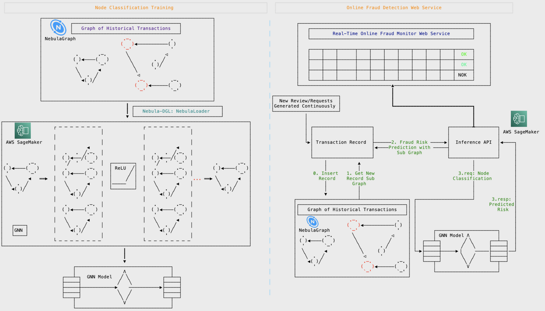
模型訓練系統(左邊):
- 輸入:帶有欺詐標註的歷史交易圖譜
- 輸出:一個 GraphSAGE 的 DGL 模型
線上推理系統(右邊):
模型:基於帶有欺詐標註的歷史交易圖譜基於 GraphSAGE 訓練
- 輸入:一筆新的交易
- 輸出:這筆交易是否涉嫌欺詐
分割資料集
機器學習訓練的過程需要在已有資料、資訊中分割出用來訓練、驗證和測試的子集。它們可以是不相交的全資料的真子集,也可以彼此有重疊的資料集。事實上,我們對資料的標註大多是不充分的,所以按照標註的比例去分割資料可能更有意義一些。下面的例子是我按照點上是否標註欺詐為標準去分割資料集。
這裡邊有兩個地方值得注意:
train_test_split 中的 stratify=g.ndata['is_fraud'] 代表保持 is_fraud 的值的分佈去分割,符合我們前面提到的思想。
我們分割的是 idx 索引,這樣,可以最終獲得三個集合的索引,供訓練、驗證和測試時候使用。同時,我們還把對應集合 mask 放到圖物件 g 裡邊去了。
# Split the graph into train, validation, and test sets

import pandas as pd
import numpy as np
from sklearn.model_selection import train_test_split

# features are g.ndata['f0'], g.ndata['f1'], g.ndata['f2'], ... g.ndata['f31']
# label is in g.ndata['is_fraud']

# concatenate all features
features = []
for i in range(32):
    features.append(g.ndata['f' + str(i)])

g.ndata['feat'] = torch.stack(features, dim=1)
g.ndata['label'] = g.ndata['is_fraud']
# numpy array as an index of range n

idx = torch.tensor(np.arange(g.number_of_nodes()), device=device, dtype=torch.int64)

# split based on value distribution of label: the property "is_fraud", which is a binary variable.
X_train_and_val_idx, X_test_idx, y_train_and_val, y_test = train_test_split(
    idx, g.ndata['is_fraud'], test_size=0.2, random_state=42, stratify=g.ndata['is_fraud'])

# split train and val
X_train_idx, X_val_idx, y_train, y_val = train_test_split(
    X_train_and_val_idx, y_train_and_val, test_size=0.2, random_state=42, stratify=y_train_and_val)

# list of index to mask
train_mask = torch.zeros(g.number_of_nodes(), dtype=torch.bool)
train_mask[X_train_idx] = True

val_mask = torch.zeros(g.number_of_nodes(), dtype=torch.bool)
val_mask[X_val_idx] = True

test_mask = torch.zeros(g.number_of_nodes(), dtype=torch.bool)
test_mask[X_test_idx] = True

g.ndata['train_mask'] = train_mask
g.ndata['val_mask'] = val_mask
g.ndata['test_mask'] = test_mask
異構圖轉換為同構圖
GraphSAGE 是針對同構圖且邊無 feature 的演演算法,而我們當下的 Yelp 圖譜是異構的:一類點、三類邊。那麼,如何才能用 GraphSAGE 去建模 Yelp 圖譜呢?
我們除了選擇用針對異構圖的 Inductive Learning 方法之外,還可想辦法把同構圖轉換成異構圖。為了在轉換中不丟失重要的邊型別資訊,我們可以把邊型別變成數值。
這裡我給了一維的 edge feature,當然二維(3-1 維)表示也是可以的。
# shares_restaurant_in_one_month_with: 1, b"001"
# shares_restaurant_rating_with: 2, b"010"
# shares_user_with: 4, b"100"
其實如果想用 0, 1, 2 這樣的分佈,轉換到同構圖之後的 hg.edata['_TYPE'] 也是可以直接拿來用的,詳見 https://docs.dgl.ai/en/0.9.x/generated/dgl.to_homogeneous.html 中的例子。
程式碼如下:
# three types of edges
In [1]: g.etypes
Out[1]:
['shares_restaurant_in_one_month_with',
 'shares_restaurant_rating_with',
 'shares_user_with']

In [2]:
g.edges['shares_restaurant_in_one_month_with'].data['he'] = torch.ones(
    g.number_of_edges('shares_restaurant_in_one_month_with'), dtype=torch.int64)
g.edges['shares_restaurant_rating_with'].data['he'] = torch.full(
    (g.number_of_edges('shares_restaurant_rating_with'),), 2, dtype=torch.int64)
g.edges['shares_user_with'].data['he'] = torch.full(
    (g.number_of_edges('shares_user_with'),), 4, dtype=torch.int64)

In [3]: g.edata['he']
Out[3]:
{('review',
  'shares_restaurant_in_one_month_with',
  'review'): tensor([1, 1, 1,  ..., 1, 1, 1]),
 ('review',
  'shares_restaurant_rating_with',
  'review'): tensor([2, 2, 2,  ..., 2, 2, 2]),
 ('review', 'shares_user_with', 'review'): tensor([4, 4, 4,  ..., 4, 4, 4])}
將它轉換為同構圖,把 he 作為要保留的 edata:
hg = dgl.to_homogeneous(g, edata=['he'], ndata=['feat', 'label', 'train_mask', 'val_mask', 'test_mask'])預設的 GraphSAGE 實現是沒考慮 edge feature 的,我們要修改訊息傳遞的步驟,在後邊會涉及到這部分的實操。
模型訓練程式碼
DGL 官方在 https://github.com/dmlc/dgl/tree/master/examples/pytorch/graphsage 給出了 GraphSAGE 例子,我在測試時修復了一個小 bug。
因為我們處理過的同構圖帶有 edge feature,不能照搬官方的 GraphSAGE 例子程式碼,我們有兩種方法來處理它:
- 可以稍微改動一下
SAGEConv訊息傳遞的部分,以 mean 聚合的方式為例:
  graph.update_all(msg_fn, fn.mean('m', 'neigh'))
+ graph.update_all(fn.copy_e('he', 'm'), fn.mean('m', 'neigh'))
- h_neigh = graph.dstdata['neigh']
+ h_neigh = torch.cat((graph.dstdata['neigh'], graph.dstdata['neigh_e'].reshape(-1, 1)), 1)
這個處理中,除了上邊訊息傳遞部分增加 edge feature 之外,還需要注意 feature 維度的處理。
- 把邊引數作為邊權重,以 mean 聚合為例:
- graph.update_all(msg_fn, fn.mean('m', 'neigh'))
+ # consdier datatype with different weight, g.edata['he'] as weight here
+ g.update_all(fn.u_mul_e('h', 'he', 'm'), fn.mean('m', 'h'))
下面,我們以把邊的型別作為權重的方式,mean 作為聚合的情況為例來實操:
我們來繼承並覆蓋 SAGEConv,其實只是修改 Message Passing 的部分:
from dgl import function as fn
from dgl.utils import check_eq_shape, expand_as_pair

class SAGEConv(dglnn.SAGEConv):
    def forward(self, graph, feat, edge_weight=None):
        r"""

        Description
        -----------
        Compute GraphSAGE layer.

        Parameters
        ----------
        graph : DGLGraph
            The graph.
        feat : torch.Tensor or pair of torch.Tensor
            If a torch.Tensor is given, it represents the input feature of shape
            :math:`(N, D_{in})`
            where :math:`D_{in}` is size of input feature, :math:`N` is the number of nodes.
            If a pair of torch.Tensor is given, the pair must contain two tensors of shape
            :math:`(N_{in}, D_{in_{src}})` and :math:`(N_{out}, D_{in_{dst}})`.
        edge_weight : torch.Tensor, optional
            Optional tensor on the edge. If given, the convolution will weight
            with regard to the message.

        Returns
        -------
        torch.Tensor
            The output feature of shape :math:`(N_{dst}, D_{out})`
            where :math:`N_{dst}` is the number of destination nodes in the input graph,
            :math:`D_{out}` is the size of the output feature.
        """
        self._compatibility_check()
        with graph.local_scope():
            if isinstance(feat, tuple):
                feat_src = self.feat_drop(feat[0])
                feat_dst = self.feat_drop(feat[1])
            else:
                feat_src = feat_dst = self.feat_drop(feat)
                if graph.is_block:
                    feat_dst = feat_src[:graph.number_of_dst_nodes()]
            msg_fn = fn.copy_src('h', 'm')
            if edge_weight is not None:
                assert edge_weight.shape[0] == graph.number_of_edges()
                graph.edata['_edge_weight'] = edge_weight
                msg_fn = fn.u_mul_e('h', '_edge_weight', 'm')

            h_self = feat_dst

            # Handle the case of graphs without edges
            if graph.number_of_edges() == 0:
                graph.dstdata['neigh'] = torch.zeros(
                    feat_dst.shape[0], self._in_src_feats).to(feat_dst)

            # Determine whether to apply linear transformation before message passing A(XW)
            lin_before_mp = self._in_src_feats > self._out_feats

            # Message Passing
            if self._aggre_type == 'mean':
                graph.srcdata['h'] = self.fc_neigh(feat_src) if lin_before_mp else feat_src
                # graph.update_all(msg_fn, fn.mean('m', 'neigh'))
                #########################################################################
                # consdier datatype with different weight, g.edata['he'] as weight here
                g.update_all(fn.u_mul_e('h', 'he', 'm'), fn.mean('m', 'h'))
                #########################################################################
                h_neigh = graph.dstdata['neigh']
                if not lin_before_mp:
                    h_neigh = self.fc_neigh(h_neigh)
            elif self._aggre_type == 'gcn':
                check_eq_shape(feat)
                graph.srcdata['h'] = self.fc_neigh(feat_src) if lin_before_mp else feat_src
                if isinstance(feat, tuple):  # heterogeneous
                    graph.dstdata['h'] = self.fc_neigh(feat_dst) if lin_before_mp else feat_dst
                else:
                    if graph.is_block:
                        graph.dstdata['h'] = graph.srcdata['h'][:graph.num_dst_nodes()]
                    else:
                        graph.dstdata['h'] = graph.srcdata['h']
                graph.update_all(msg_fn, fn.sum('m', 'neigh'))
                graph.update_all(fn.copy_e('he', 'm'), fn.sum('m', 'neigh'))
                # divide in_degrees
                degs = graph.in_degrees().to(feat_dst)
                h_neigh = (graph.dstdata['neigh'] + graph.dstdata['h']) / (degs.unsqueeze(-1) + 1)
                if not lin_before_mp:
                    h_neigh = self.fc_neigh(h_neigh)
            elif self._aggre_type == 'pool':
                graph.srcdata['h'] = F.relu(self.fc_pool(feat_src))
                graph.update_all(msg_fn, fn.max('m', 'neigh'))
                graph.update_all(fn.copy_e('he', 'm'), fn.max('m', 'neigh'))
                h_neigh = self.fc_neigh(graph.dstdata['neigh'])
            elif self._aggre_type == 'lstm':
                graph.srcdata['h'] = feat_src
                graph.update_all(msg_fn, self._lstm_reducer)
                h_neigh = self.fc_neigh(graph.dstdata['neigh'])
            else:
                raise KeyError('Aggregator type {} not recognized.'.format(self._aggre_type))

            # GraphSAGE GCN does not require fc_self.
            if self._aggre_type == 'gcn':
                rst = h_neigh
            else:
                rst = self.fc_self(h_self) + h_neigh

            # bias term
            if self.bias is not None:
                rst = rst + self.bias

            # activation
            if self.activation is not None:
                rst = self.activation(rst)
            # normalization
            if self.norm is not None:
                rst = self.norm(rst)
            return rst
定義模型:
class SAGE(nn.Module):
    def __init__(self, in_size, hid_size, out_size):
        super().__init__()
        self.layers = nn.ModuleList()
        # three-layer GraphSAGE-mean
        self.layers.append(dglnn.SAGEConv(in_size, hid_size, 'mean'))
        self.layers.append(dglnn.SAGEConv(hid_size, hid_size, 'mean'))
        self.layers.append(dglnn.SAGEConv(hid_size, out_size, 'mean'))
        self.dropout = nn.Dropout(0.5)
        self.hid_size = hid_size
        self.out_size = out_size

    def forward(self, blocks, x):
        h = x
        for l, (layer, block) in enumerate(zip(self.layers, blocks)):
            h = layer(block, h)
            if l != len(self.layers) - 1:
                h = F.relu(h)
                h = self.dropout(h)
        return h

    def inference(self, g, device, batch_size):
        """Conduct layer-wise inference to get all the node embeddings."""
        feat = g.ndata['feat']
        sampler = MultiLayerFullNeighborSampler(1, prefetch_node_feats=['feat'])
        dataloader = DataLoader(
                g, torch.arange(g.num_nodes()).to(g.device), sampler, device=device,
                batch_size=batch_size, shuffle=False, drop_last=False,
                num_workers=0)
        buffer_device = torch.device('cpu')
        pin_memory = (buffer_device != device)

        for l, layer in enumerate(self.layers):
            y = torch.empty(
                g.num_nodes(), self.hid_size if l != len(self.layers) - 1 else self.out_size,
                device=buffer_device, pin_memory=pin_memory)
            feat = feat.to(device)
            for input_nodes, output_nodes, blocks in tqdm.tqdm(dataloader):
                x = feat[input_nodes]
                h = layer(blocks[0], x) # len(blocks) = 1
                if l != len(self.layers) - 1:
                    h = F.relu(h)
                    h = self.dropout(h)
                # by design, our output nodes are contiguous
                y[output_nodes[0]:output_nodes[-1]+1] = h.to(buffer_device)
            feat = y
        return y
定義訓練、推理的函式:
def evaluate(model, graph, dataloader):
    model.eval()
    ys = []
    y_hats = []
    for it, (input_nodes, output_nodes, blocks) in enumerate(dataloader):
        with torch.no_grad():
            x = blocks[0].srcdata['feat']
            ys.append(blocks[-1].dstdata['label'])
            y_hats.append(model(blocks, x))
    return MF.accuracy(torch.cat(y_hats), torch.cat(ys))

def layerwise_infer(device, graph, nid, model, batch_size):
    model.eval()
    with torch.no_grad():
        pred = model.inference(graph, device, batch_size) # pred in buffer_device
        pred = pred[nid]
        label = graph.ndata['label'][nid].to(pred.device)
        return MF.accuracy(pred, label)

def train(device, g, model, train_idx, val_idx):
    # create sampler & dataloader
    sampler = NeighborSampler([10, 10, 10],  # fanout for [layer-0, layer-1, layer-2]
                              prefetch_node_feats=['feat'],
                              prefetch_labels=['label'])
    use_uva = False
    train_dataloader = DataLoader(g, train_idx, sampler, device=device,
                                  batch_size=1024, shuffle=True,
                                  drop_last=False, num_workers=0,
                                  use_uva=use_uva)

    val_dataloader = DataLoader(g, val_idx, sampler, device=device,
                                batch_size=1024, shuffle=True,
                                drop_last=False, num_workers=0,
                                use_uva=use_uva)

    opt = torch.optim.Adam(model.parameters(), lr=1e-3, weight_decay=5e-4)

    for epoch in range(10):
        model.train()
        total_loss = 0
        for it, (input_nodes, output_nodes, blocks) in enumerate(train_dataloader):
            x = blocks[0].srcdata['feat']
            y = blocks[-1].dstdata['label']
            y_hat = model(blocks, x)
            loss = F.cross_entropy(y_hat, y)
            opt.zero_grad()
            loss.backward()
            opt.step()
            total_loss += loss.item()
        acc = evaluate(model, g, val_dataloader)
        print("Epoch {:05d} | Loss {:.4f} | Accuracy {:.4f} "
              .format(epoch, total_loss / (it+1), acc.item()))
從 NebulaGraph 中載入圖到 DGL,得到的是一個異構圖(一類點、三類邊):
from nebula_dgl import NebulaLoader

nebula_config = {
    "graph_hosts": [
                ('graphd', 9669),
                ('graphd1', 9669),
                ('graphd2', 9669)
            ],
    "nebula_user": "root",
    "nebula_password": "nebula",
}

with open('nebulagraph_yelp_dgl_mapper.yaml', 'r') as f:
     feature_mapper = yaml.safe_load(f)

nebula_loader = NebulaLoader(nebula_config, feature_mapper)

g = nebula_loader.load() # This will take you some time

# 作為窮人,我們用 CPU
g = g.to('cpu')
device = torch.device('cpu')
分出訓練、驗證、測試集,再轉換成同構圖:
# Split the graph into train, validation and test sets

import pandas as pd
import numpy as np
from sklearn.model_selection import train_test_split

# features are g.ndata['f0'], g.ndata['f1'], g.ndata['f2'], ... g.ndata['f31']
# label is in g.ndata['is_fraud']

# concatenate all features
features = []
for i in range(32):
    features.append(g.ndata['f'+str(i)])

g.ndata['feat'] = torch.stack(features, dim=1)
g.ndata['label'] = g.ndata['is_fraud']
# numpy array as index of range n

idx = torch.tensor(np.arange(g.number_of_nodes()), device=device, dtype=torch.int64)
# features.append(idx)
# concatenate one dim with index of node
# feature_and_idx = torch.stack(features, dim=1)

# split based on value distribution of label: the property "is_fraud", which is a binary variable.
X_train_and_val_idx, X_test_idx, y_train_and_val, y_test = train_test_split(
    idx, g.ndata['is_fraud'], test_size=0.2, random_state=42, stratify=g.ndata['is_fraud'])

# split train and val
X_train_idx, X_val_idx, y_train, y_val = train_test_split(
    X_train_and_val_idx, y_train_and_val, test_size=0.2, random_state=42, stratify=y_train_and_val)

# list of index to mask
train_mask = torch.zeros(g.number_of_nodes(), dtype=torch.bool)
train_mask[X_train_idx] = True

val_mask = torch.zeros(g.number_of_nodes(), dtype=torch.bool)
val_mask[X_val_idx] = True

test_mask = torch.zeros(g.number_of_nodes(), dtype=torch.bool)
test_mask[X_test_idx] = True

g.ndata['train_mask'] = train_mask
g.ndata['val_mask'] = val_mask
g.ndata['test_mask'] = test_mask

# shares_restaurant_in_one_month_with: 1, b"001"
# shares_restaurant_rating_with: 2, b"010"
# shares_user_with: 4, b"100"
# set edata of shares_restaurant_in_one_month_with to n of 1 tensor array
g.edges['shares_restaurant_in_one_month_with'].data['he'] = torch.ones(
    g.number_of_edges('shares_restaurant_in_one_month_with'), dtype=torch.float32)
g.edges['shares_restaurant_rating_with'].data['he'] = torch.full(
    (g.number_of_edges('shares_restaurant_rating_with'),), 2, dtype=torch.float32)
g.edges['shares_user_with'].data['he'] = torch.full(
    (g.number_of_edges('shares_user_with'),), 4, dtype=torch.float32)

# heterogeneous graph to heterogeneous graph, keep ndata and edata
hg = dgl.to_homogeneous(g, edata=['he'], ndata=['feat', 'label', 'train_mask', 'val_mask', 'test_mask'])
訓練、測試模型:
# create GraphSAGE model
in_size = hg.ndata['feat'].shape[1]
out_size = 2
model = SAGE(in_size, 256, out_size).to(device)

# model training
print('Training...')
train(device, hg, model, X_train_idx, X_val_idx)

# test the model
print('Testing...')

acc = layerwise_infer(device, hg, X_test_idx, model, batch_size=4096)
print("Test Accuracy {:.4f}".format(acc.item()))

# 執行結果
# Test Accuracy 0.9996
有了模型之後,我們可以把它序列化成檔案,在需要的時候,只需要把模型的形式和這個序列化檔案再載入成一個 pyTorch 就可以用它進行推理了。
# save model
torch.save(model.state_dict(), "fraud_d.model")

# load model
device = torch.device('cpu')
model = SAGE(32, 256, 2).to(device)
model.load_state_dict(torch.load("fraud_d.model"))
最後,我們如何把模型放到我們的線上欺詐檢測系統裡呢?
推理介面
前邊提到過,GraphSAGE 是最簡單的支援 Inductive Learning 的模型。但上面我們的訓練推理用的圖和測試是同一張,而 Inductive Learning 最佳態是推理所用資料為全新點、邊。為了做到 Inductive Learning,我們只需要把訓練和測試分成兩個無交集的子圖來做訓練和最終測試:
# Inductive Learning, our test dataset are new nodes and new edges
hg_train = hg.subgraph(torch.cat([X_train_idx, X_val_idx]))

# model training
print('Training...')
train(device, hg_train, model, torch.arange(X_train_idx.shape[0]), torch.arange(X_train_idx.shape[0], hg_train.num_nodes()))

# test the model
print('Testing...')

hg_test = hg.subgraph(torch.cat([X_test_idx]))

sg_X_test_idx = torch.arange(hg_test.num_nodes())

acc = layerwise_infer(device, hg_test, sg_X_test_idx, model, batch_size=4096)
print("Test Accuracy {:.4f}".format(acc.item()))

# 執行結果
# Test Accuracy 0.9990
可以看到,我們上面的程式碼裡,測試所用到的圖和訓練的圖是完全不同的兩組資料,這使得我們的線上系統可以遇到之前完全沒有碰到過的資料。只要把新的交易請求資料寫進 NebulaGraph,再從這個點獲取一個線上系統可以返回的小子圖,就可以把它作為模型推理的輸入,獲得子圖的標籤了!
新的交易請求
還記得我們前邊畫的線上推理系統的流程圖麼?
      ┌─────────────────────┐                          ┌─────────────────┐
      │                     │                          │                 │
─────▶│ Transaction Record  ├──────2. Fraud Risk ─────▶│  Inference API  │◀────┐
      │                     │◀────Prediction with ─────┤                 │     │
      │                     │        Sub Graph         │                 │     │
      └─────────────────────┘                          └─────────────────┘     │
           │           ▲                                        │              │
           │           │                                        │              │
       0. Insert   1. Get New                              3.req: Node         │
         Record    Record Sub                            Classification        │
           │         Graph                                      │              │
           ▼           │                                        │              │
┌──────────────────────┴─────────────────┐ ┌────────────────────┘      3.resp: │
│┌──────────────────────────────────────┐│ │                          Predicted│
││   Graph of Historical Transactions   ││ │                             Risk  │
│└──────────────────────────────────────┘│ │                                   │
│                   .─.              .   │ │                                   │
│                  (   )◀───────────( )  │ │                                   │
│                   `─'              '   │ │      ┌──────────────────────┐     │
│  .       .─.       ╲             ◁     │ │      │ GNN Model Λ          │     │
│ ( )◀────(   )       ╲           ╱      │ │  ┌───┴─┐        ╱ ╲      ┌──┴──┐  │
│  '       `─'         ╲       . ╱       │ │  ├─────┤       ╱   ╲     ├─────┤  │
│  ╲       ◀            ╲     ( )        │ └─▶├─────┼─────▶▕     ─────├─────┤──┘
│   ╲  .  ╱              ◁     '         │    ├─────┤       ╲   ╱     ├─────┤
│    ◀( )╱               .─.         .─. │    └───┬─┘        ╲ ╱      └──┬──┘
│      '                (   )◀──────(   )│        │           V          │
│                        `─'         `─' │        └──────────────────────┘
└────────────────────────────────────────┘
現在,我們假設這個新的交易請求已經發起,這條交易記錄已經被更新在圖譜裡,我們們隨便取一個點作為這樣的請求吧。
MATCH (n:review) RETURN n LIMIT 1+----------------------------------------------------------------------------------------------------------------------------------------------------------------------------------------------------------------------------------------------------------------------------------------------------------------------------------------------------------------------------------------------------------------------------------------------------------------------------------------------------------------------------------------------------------------------------------------------------------------------------------------------------------------------------------------------------------------------------------------------------------------------------------------------------------------------------------------+
| n |
+----------------------------------------------------------------------------------------------------------------------------------------------------------------------------------------------------------------------------------------------------------------------------------------------------------------------------------------------------------------------------------------------------------------------------------------------------------------------------------------------------------------------------------------------------------------------------------------------------------------------------------------------------------------------------------------------------------------------------------------------------------------------------------------------------------------------------------------+
| (2048 :review{f0: 0.0, f1: 0.08034700155258179, f10: 0.3952670097351074, f11: 0.18671999871730804, f12: 0.2836120128631592, f13: 0.2843089997768402, f14: 0.38148200511932373, f15: 0.3816460072994232, f16: 0.9999740123748779, f17: 0.6430919766426086, f18: 0.9999740123748779, f19: 0.5051100254058838, f2: 0.12382200360298157, f20: 0.4940490126609802, f21: 0.7766339778900146, f22: 0.7705119848251343, f23: 0.9480599761009216, f24: 0.4032529890537262, f25: 0.12437800318002701, f26: 0.3184080123901367, f27: 0.5223879814147949, f28: 0.4278610050678253, f29: 0.343284010887146, f3: 0.42868199944496155, f30: 0.37313398718833923, f31: 0.328357994556427, f4: 0.9999849796295166, f5: 0.9999849796295166, f6: 0.9999849796295166, f7: 0.4850809872150421, f8: 0.454602986574173, f9: 0.8863419890403748, is_fraud: 0}) |
+----------------------------------------------------------------------------------------------------------------------------------------------------------------------------------------------------------------------------------------------------------------------------------------------------------------------------------------------------------------------------------------------------------------------------------------------------------------------------------------------------------------------------------------------------------------------------------------------------------------------------------------------------------------------------------------------------------------------------------------------------------------------------------------------------------------------------------------+好,它是 2048 這個點。
它的下一步是 1. Get New Record Subgraph 我們來獲取它的子圖:
GET SUBGRAPH WITH PROP FROM 2048 YIELD VERTICES AS nodes, EDGES AS relationships;可以看到返回的結果其實還是很多的,btw 在 NebulaGraph 中這個子圖結果返回獲取是在 10 ms 左右。假若,這裡我們使用圖視覺化探索工具 NebulaGraph Studio 或者 Explorer,可以把結果渲染出來(視覺化展示的 Query 可以去掉 WITH PROP ,可以給瀏覽器省點記憶體),結果就更容易讓人腦理解了:


現在,我們就來實現這一步的程式碼吧。它的輸入是點的 id:vertex_id,輸出是一個 dgl_graph,用來傳給推理介面。
# get SUBGRAPH of one node

import json
from torch import tensor
from dgl import DGLHeteroGraph, heterograph

from nebula3.gclient.net import ConnectionPool
from nebula3.Config import Config

config = Config()
config.max_connection_pool_size = 2
connection_pool = ConnectionPool()
connection_pool.init([('graphd', 9669)], config)

vertex_id = 2048
client = connection_pool.get_session('root', 'nebula')
r = client.execute_json(
    "USE yelp;"
    f"GET SUBGRAPH WITH PROP 2 STEPS FROM {vertex_id} YIELD VERTICES AS nodes, EDGES AS relationships;")

r = json.loads(r)
data = r.get('results', [{}])[0].get('data')
這裡我用到了 nebula-python,這個 NebulaGraph 的 Python SDK/Client。透過 execute_json 執行獲得了這個交易的子圖。
下一步,我們們需要把它構造成一個 dgl_graph:
# create node and nodedata
node_id_map = {} # key: vertex id in NebulaGraph, value: node id in dgl_graph
node_idx = 0
features = [[] for _ in range(32)] + [[]]
for i in range(len(data)):
    for index, node in enumerate(data[i]['meta'][0]):
        nodeid = data[i]['meta'][0][index]['id']
        if nodeid not in node_id_map:
            node_id_map[nodeid] = node_idx
            node_idx += 1
            for f in range(32):
                features[f].append(data[i]['row'][0][index][f"review.f{f}"])
            features[32].append(data[i]['row'][0][index]['review.is_fraud'])


"""
- R-U-R:兩個評價由同一個使用者發出 shares_user_with
- R-S-R:兩個評價是同餐廳同評分(評分可以是1到5) shares_restaurant_rating_with
- R-T-R:兩個評價是同餐廳同提交月份 shares_restaurant_in_one_month_with
"""
rur_start, rur_end, rsr_start, rsr_end, rtr_start, rtr_end = [], [], [], [], [], []
for i in range(len(data)):
    for edge in data[i]['meta'][1]:
        edge = edge['id']
        if edge['name'] == 'shares_user_with':
            rur_start.append(node_id_map[edge['src']])
            rur_end.append(node_id_map[edge['dst']])
        elif edge['name'] == 'shares_restaurant_rating_with':
            rsr_start.append(node_id_map[edge['src']])
            rsr_end.append(node_id_map[edge['dst']])
        elif edge['name'] == 'shares_restaurant_in_one_month_with':
            rtr_start.append(node_id_map[edge['src']])
            rtr_end.append(node_id_map[edge['dst']])

data_dict = {}
if rur_start:
    data_dict[('review', 'shares_user_with', 'review')] = tensor(rur_start), tensor(rur_end)
if rsr_start:
    data_dict[('review', 'shares_restaurant_rating_with', 'review')] = tensor(rsr_start), tensor(rsr_end)
if rtr_start:
    data_dict[('review', 'shares_restaurant_in_one_month_with', 'review')] = tensor(rtr_start), tensor(rtr_end)

# construct a dgl_graph
dgl_graph: DGLHeteroGraph = heterograph(data_dict)
實際上我就是按照 DGL 檔案 https://docs.dgl.ai/en/0.9.x/generated/dgl.heterograph.html 中的方式去構造 data_dict。再用 heterograph() 就把結果轉換為想要的 dgl_graph 了,其中 node_id_map 是 NebulaGraph 之中 Vertex_ID 到這個物件中 node_id 的字典。
最後,我們再把 node feature 也載入進去。
# load node features to dgl_graph
for i in range(32):
    dgl_graph.ndata[f"f{i}"] = tensor(features[i])
dgl_graph.ndata['label'] = tensor(features[32])
在開始推理之前,我們還需要把它轉換成同構圖,和前面完全一樣:
import torch


# to homogeneous graph
features = []
for i in range(32):
    features.append(dgl_graph.ndata[f"f{i}"])

dgl_graph.ndata['feat'] = torch.stack(features, dim=1)

dgl_graph.edges['shares_restaurant_in_one_month_with'].data['he'] = torch.ones(
    dgl_graph.number_of_edges('shares_restaurant_in_one_month_with'), dtype=torch.float32)
dgl_graph.edges['shares_restaurant_rating_with'].data['he'] = torch.full(
    (dgl_graph.number_of_edges('shares_restaurant_rating_with'),), 2, dtype=torch.float32)
dgl_graph.edges['shares_user_with'].data['he'] = torch.full(
    (dgl_graph.number_of_edges('shares_user_with'),), 4, dtype=torch.float32)


# heterogeneous graph to heterogeneous graph, keep ndata and edata
import dgl
hg = dgl.to_homogeneous(dgl_graph, edata=['he'], ndata=['feat', 'label'])
最後,我們的推理介面就是:
def do_inference(device, graph, node_idx, model, batch_size):
    model.eval()
    with torch.no_grad():
        pred = model.inference(graph, device, batch_size) # pred in buffer_device
        return pred[node_idx]
我們可以呼叫一下試試推理我們這個新的點:
node_idx = node_id_map[vertex_id]
batch_size = 4096

result = do_inference(device, hg, node_idx, model, batch_size)
當然,我們也能在這個小子圖上計算它的正確率:
def test_inference(device, graph, nid, model, batch_size):
    model.eval()
    with torch.no_grad():
        pred = model.inference(graph, device, batch_size) # pred in buffer_device
        pred = pred[nid]
        label = graph.ndata['label'][nid].to(pred.device)
        return MF.accuracy(pred, label)

node_idx = torch.tensor(list(node_id_map.values()))
acc = test_inference(device, hg, node_idx, model, batch_size=4096)
print("Test Accuracy {:.4f}".format(acc.item()))
輸出結果:
In [307]: def test_inference(device, graph, nid, model, batch_size):
     ...:     model.eval()
     ...:     with torch.no_grad():
     ...:         pred = model.inference(graph, device, batch_size) # pred in buffer
     ...: _device
     ...:         pred = pred[nid]
     ...:         label = graph.ndata['label'][nid].to(pred.device)
     ...:         return MF.accuracy(pred, label)
     ...:
     ...: node_idx = torch.tensor(list(node_id_map.values()))
     ...: acc = test_inference(device, hg, node_idx, model, batch_size=4096)
     ...: print("Test Accuracy {:.4f}".format(acc.item()))
     ...:
100%|████████████████████████████████████████████████| 1/1 [00:00<00:00, 130.31it/s]
100%|████████████████████████████████████████████████| 1/1 [00:00<00:00, 152.29it/s]
100%|████████████████████████████████████████████████| 1/1 [00:00<00:00, 173.55it/s]
Test Accuracy 0.9688這個示例專案的程式碼在:github.com/wey-gu/NebulaGraph-Fraud-Detection-GNN ,如有問題歡迎留言、issue 一起交流。
AWS 上生產級別落地參考解決方案
前文的例項都是在最小的實驗環境中可操作、可復現的方案。本節針對生產落地進行簡短的討論,並給出了 AWS 上的示例參考架構。
注:可以從這個連結瞭解 NebulaGraph on AWS:https://aws.amazon.com/quickstart/architecture/vesoft-nebula-graph/
基於圖譜與專家圖模式匹配方法
本方法本質是一個基於 NebulaGraph 的圖譜 OLTP 應用,推薦的生產落地方案是基於 NebulaGraph on AWS。
如下圖所示,NebulaGraph on AWS 在 AWS 的基礎設施之上,由 NebulaGraph 主要支援團隊(Vesoft Inc.)提供了開箱即用的生產級別部署架構,與企業級圖資料庫 NebulaGraph Core Enterprise 及其配套的豐富周邊工具。
解決方案如圖所示:

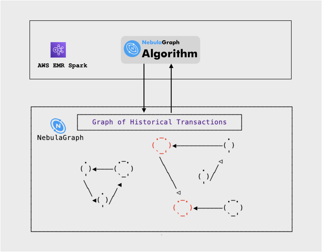
基於圖計算的方法
上面我們舉例了基於圖演演算法的擴充欺詐風險標註實踐,並用了單機的方案進行 demo。在生產環境落地時,比如 AWS 上,除了 AWS 上的 NebulaGraph 核心叢集之外,我們還需要 NebulaGraph Algorithm,後者可以執行在 AWS EMR Spark 之上,從 NebulaGraph 中抽取全圖資料,並在 Spark 叢集中分散式高效進行圖演演算法。
解決方案如圖所示:
圖神經網路的方法
此外,前邊我們利用 NebulaGraph、DGL、Nebula-DGL 的基於 GNN 的實時風控專案在 AWS 生產中可以:
- 訓練、預研使用 AWS SageMaker和 SageMaker Notebook
- 線上推理使用 AWS SageMaker Inference。其中,針對金融風控等流量按不同時段呈現較大浮動的情況,可以考慮使用 AWS SageMaker Inference Serverless,藉助其 scale to zero 同時和無線擴容的能力,做到極致的算力的按需付費
解決方案如圖所示:
總結
總結起來,欺詐檢測的方法有:
- 在一個交易歷史、風控的圖譜上,透過圖模式查詢直接獲得風險提示
- 定期利用圖演演算法擴充風險標註,寫回相簿
- 定期計算圖譜中的圖特徵,和其他特徵一起用傳統機器學習方法離線預測風險
- 將圖譜中的屬性處理成為點、邊特徵,用圖神經網路方法離線預測風險,部分可以 Inductive Learning 的方法結合相簿可以實現線上風險預測
延伸閱讀
- DGL 外部資料匯入檔案:https://docs.dgl.ai/guide/graph-external.html
- 如何將異質圖轉換為帶資料的同質圖:https://discuss.dgl.ai/t/how-to-convert-from-a-heterogeneous-graph-to-a-homogeneous-graph-with-data/2764
- https://docs.dgl.ai/en/latest/guide/graph-heterogeneous.html?highlight=to_homogeneous#converting-heterogeneous-graphs-to-homogeneous-graphs
- DGL FAQ 第 13 個問題:https://discuss.dgl.ai/t/frequently-asked-questions-faq/1681
- https://discuss.dgl.ai/t/using-node-and-edge-features-in-message-passing/762
謝謝你讀完本文 (///▽///)
要來近距離體驗一把圖資料庫嗎?現在可以用用 NebulaGraph Cloud 來搭建自己的圖資料系統喲,快來節省大量的部署安裝時間來搞定業務吧~ NebulaGraph 阿里雲端計算巢現 30 天免費使用中,點選連結來用用圖資料庫吧~
想看原始碼的小夥伴可以前往 GitHub 閱讀、使用、(^з^)-☆ star 它 -> GitHub;和其他的 NebulaGraph 使用者一起交流圖資料庫技術和應用技能,留下「你的名片」一起玩耍呢~