Caffe中的優化方法
【原文:http://demo.netfoucs.com/danieljianfeng/article/details/42931721】
在Deep Learning中,往往loss function是非凸的,沒有解析解,我們需要通過優化方法來求解。Caffe通過協調的進行整個網路的前向傳播推倒以及後向梯度對引數進行更新,試圖減小損失。
Caffe已經封裝好了三種優化方法,分別是Stochastic Gradient Descent (SGD), AdaptiveGradient (ADAGRAD), and Nesterov’s Accelerated Gradient (NAG)。
Solver的流程:
1. 設計好需要優化的物件,以及用於學習的訓練網路和用於評估的測試網路。
2. 通過forward和backward迭代的進行優化來跟新引數
3. 定期的評價測試網路
4. 在優化過程中顯示模型和solver的狀態
每一步迭代的過程
1. 通過forward計算網路的輸出和loss
2. 通過backward計算網路的梯度
3. 根據solver方法,利用梯度來對引數進行更新
4. 根據learning rate,history和method來更新solver的狀態
和Caffe模型一樣,Caffe solvers也可以CPU / GPU執行。
1. Methods
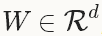
Solver方法一般用來解決loss函式的最小化問題。對於一個資料集D,需要優化的目標函式是整個資料集中所有資料loss的平均值。
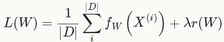
其中, r(W)是正則項,為了減弱過擬合現象。
如果採用這種Loss 函式,迭代一次需要計算整個資料集,在資料集非常大的這情況下,這種方法的效率很低,這個也是我們熟知的梯度下降採用的方法。
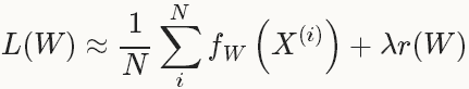
在實際中,會採用整個資料集的一個mini-batch,其數量為N<<|D|,此時的loss 函式為:
1.1 SGD
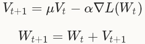
型別:SGD隨機梯度下降(Stochastic gradient descent)通過negative梯度 和上一次的權重更新值V_t的線性組合來更新W,迭代公式如下:


設定learningrate和momentum的經驗法則
例子
<span style="background-color: rgb(255, 255, 255);">base_lr: 0.01 # begin training at a learning rate of0.01 = 1e-2 lr_policy: "step" # learning ratepolicy: drop the learning rate in "steps" # by a factor of gamma everystepsize iterations gamma: 0.1 # drop the learning rate by a factor of10 # (i.e., multiply it by afactor of gamma = 0.1) stepsize: 100000 # drop the learning rate every 100K iterations max_iter: 350000 # train for 350K iterations total momentum: 0.9</span>
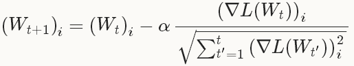
1.2 AdaGrad
型別:ADAGRAD自適應梯度(adaptive gradient)[3]是基於梯度的優化方法(like SGD),以作者的話說就是,“find needles in haystacks in the form of very predictive but rarely seen features”。給定之前所有迭代的更新資訊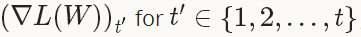 ,每一個W的第i個成分的更新如下:


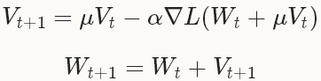
1.3 NAG
型別:NAGNesterov 的加速梯度法(Nesterov’s accelerated gradient)作為凸優化中最理想的方法,其收斂速度可以達到 而不是
而不是 。但由於深度學習中的優化問題往往是非平滑的以及非凸的(non-smoothness
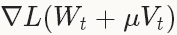
and non-convexity),在實踐中NAG對於某類深度學習的結構可以成為非常有效的優化方法,比如deep MNIST autoencoders[5]。權重的更新和SGD的的非常類似:
。但由於深度學習中的優化問題往往是非平滑的以及非凸的(non-smoothness
and non-convexity),在實踐中NAG對於某類深度學習的結構可以成為非常有效的優化方法,比如deep MNIST autoencoders[5]。權重的更新和SGD的的非常類似:
2. 參考:
[1] L. Bottou. Stochastic Gradient Descent Tricks. Neural Networks: Tricks of the Trade: Springer, 2012.[2] A. Krizhevsky, I. Sutskever, and G. Hinton. ImageNet Classification with Deep Convolutional Neural Networks. Advances in Neural Information Processing Systems, 2012.[3] J. Duchi, E. Hazan, and Y. Singer. Adaptive Subgradient Methods for Online Learning and Stochastic Optimization. The Journal of Machine Learning Research, 2011.[4] Y. Nesterov. A Method of Solving a Convex Programming Problem with Convergence Rate O(1/k√). Soviet Mathematics Doklady, 1983.[5] I. Sutskever, J. Martens, G. Dahl, and G. Hinton. On the Importance of Initialization and Momentum in Deep Learning. Proceedings of the 30th International Conference on Machine Learning, 2013.[6] http://caffe.berkeleyvision.org/tutorial/solver.html相關文章
- 深度學習中的優化方法(二)深度學習優化
- 深度學習中的優化方法(一)深度學習優化
- caffe study(4) - 優化演算法基本原理優化演算法
- Oracle優化的方法Oracle優化
- SQL優化的方法論SQL優化
- Caffe簡單例程,影像處理,Netscope視覺化方法單例視覺化
- 優化SQL中的or優化SQL
- Sql優化方法SQL優化
- Oracle優化方法Oracle優化
- union 優化方法優化
- 遊戲陪玩app開發中,Mysql的sql優化方法遊戲APPMySql優化
- 優化Angularjs的$watch方法優化AngularJS
- 不懂業務的SQL優化方法SQL優化
- SQL查詢優化的方法SQL優化
- SQL 語句的優化方法SQL優化
- Oracle資料的優化器有兩種優化方法:Oracle優化
- Oracle中的like優化Oracle優化
- iOS中responseToSelector()方法是不是需要優化iOS優化
- seo優化中不容忽視的頁面優化優化
- 【NLP】常用優化方法優化
- MySQL 優化常用方法MySql優化
- Web 效能優化方法Web優化
- 04 最優化方法優化
- Oracle效能優化方法論的發展之二:基於OWI的效能優化方法論Oracle優化
- 總結前端效能優化的方法前端優化
- PHP的效能優化方法總結PHP優化
- 運籌優化(十三)--大規模優化方法優化
- mysql 大表中count() 使用方法以及效能優化.MySql優化
- 優化MySQL中的分頁優化MySql
- 優化 MySQL 中的分頁優化MySql
- Javascript中的迴圈優化JavaScript優化
- java效能優化方案9——優化自定義hasCode()方法和equals()方法Java優化
- SQL優化常用方法11SQL優化
- SQL優化常用方法10SQL優化
- SQL優化常用方法16SQL優化
- SQL優化常用方法2SQL優化
- SQL優化常用方法5SQL優化
- SQL優化常用方法8SQL優化