Multiple Regression

Multiple Regression

What is multiple regression?

Multiple regression is regression analysis with more than one independent variable. It is used to quantify the influence of two or more independent variables on a dependent variable.
The general multiple linear regression model is:

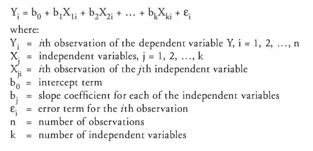
The multiple regression methodology estimates the intercept and slope coefficients such that the sum of the squared error terms,

is minimized.

The result of this procedure is the following regression equation:

Interpret Estimated Regression Coefficients and Their p-values

• The intercept term is the value of the dependent variable when the independent variables are all equal to zero.
• Each slope coefficient is the estimated change in the dependent variable for a one-unit change in that independent variable, holding the other independent variables constant. That's why the slope coefficients in a multiple regression are sometimes called partial slope coefficients.

Hypothesis Testing of Regression Coefficients

The magnitude of coefficients in a multiple regression tells us nothing about the importance of the independent variable in explaining the dependent variable. Thus, we must conduct hypothesis testing on the estimated slope coefficients to determine if the independent variables make a significant contribution to explaining the variation in the dependent variable.

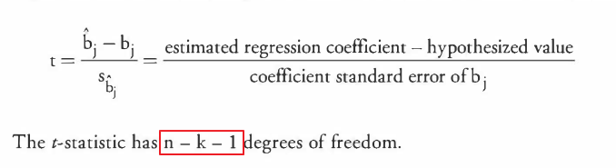
The t-statistic used to test the significance of the individual coefficients in a multiple regression is calculated using the same formula that is used with simple linear regression:

Determining Statistical Significance

The most common hypothesis test done on the regression coefficients is to test statistical significance, which means testing the null hypothesis that the coefficient is zero versus the alternative that it is not:

Interpreting p-Values

The p-value is the smallest level of significance for which the null hypothesis can be rejected. An alternative method of doing hypothesis testing of the coefficients is to compare the p-value to the significance level:

• If the p-value is less than the significance level, the null hypothesis can be rejected.
• If the p-value is greater than the significance level, the null hypothesis cannot be rejected.

Confidence Intervals for a Regression Coefficient

The confidence interval for a regression coefficient in multiple regression is calculated and interpreted the same way as it is in simple linear regression. For example, a 95% confidence interval is constructed as follows:

The critical t-value is a two tailed value with n-k-1 degrees of freedom and a 5% significance level, where n is the number of observations and k is the number of independent variables.

Note: Constructing a confidence interval and conducting a t-test with a null hypothesis of "equal to zero" will always result in the same conclusion regarding the statistical significance of the regression coefficient.

Predicating the Dependent Variable

The predicated value of dependent variable Y is:

Note: The predication of the dependent variable uses the estimated intercept and all of the estimated slope coefficients, regardless of whether the estimated coefficients are statistically significantly different from 0.

Assumption of a Multiple Regression Model

• A linear relationship exists between the dependent and independent variables.
• The independent variables are not random, and there is no exact linear relation between any two or more independent variables.

• The expected value of the error term, conditional on the independent variable, is zero.

• The variance of the error term is constant for all observations.

• The error term for one observation is not correlated with that of another observation.

• The error term is normally distributed.

The F-Statistic

An F-test assesses how well the set of independent variables, as a group, explains the variation in the dependent variable. That is, the F-statistic is used to test whether at least one of the independent variables explains a significant portion of the variation of the dependent variable.

For example, if there are 4 independent variables in the model, the hypotheses are structured as:

The F-statistic, which is always one-tailed test, is calculated as:

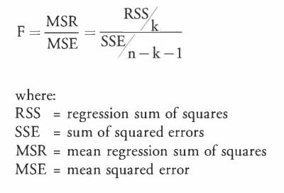
To determine whether at least one of the coefficients is statistically significant, the calculated F-statistic is compared with the one-tailed critical F-value, at the appropriate level of significance. The degrees of freedom for the numerator and denominator are:

The decision rule for the F-test is:

Rejection of the null hypothesis at a stated level of significance indicates that at least one of the coefficients is significantly different than zero, which is interpreted to mean that at least one of the independent variables in the regression model makes a significant contribution to the explanation of the dependent variable.

Note: It may have occurred to you that an easier way to test all of the coefficients simultaneously is to just conduct all the individual t-tests and see how many of them you can reject. This is the wrong approach, because if you set the significant level for each t-test at 5%, for example, the significance level from testing them all simultaneously is NOT 5%, but some higher percentage.

When testing the hypothesis that all the regression coefficients are simultaneously equal to zero, the F-test is always a one-tailed test, despite the fact that it looks like it should be a two-tailed test because there is an equal sign in the null hypothesis.

Coefficient of Determination, R^2

In addition to an F-test, the multiple coefficient of determination, R^2, can be used to test the overall effectiveness of the entire set of independent variables in explaining the dependent variable. Its interpretation is similar to that for simple linear regression: the percentage of variation in the dependent variable that is collectively explained by all of the independent variables. For example, an R^2 of 0.63 indicates that the model, as a whole, explains 63% of the variation in the dependent variable.

R^2 is also calculated the same way as in simple linear regression.

Multiple R

Regression output often includes multiple R, which is the correlation between actual values of y and forecasted values of y. Multiple R is the square root of R^2. For a regression with one independent variable, the correlation between the independent variable and dependent variable is the same as multiple R(with the sign for the slope efficient).

Adjusted R^2

Unfortunately, R^2, by itself may not be a reliable measure of the explanatory power of the multiple regression model. This is because R^2 is almost always increases as variables are added to the model, even if the marginal contribution of the new variables is not statistically significant. Consequently, a relatively high R^2 may reflect the impact of a large set of independent variables rather than how well the set explains the dependent variable. This problem is often referred to as overestimating the regression.

To overcome the problem of overestimating the impact of the additional variables on the explanatory power of a regression model, many researcher recommend adjusted R^2 for the number of independent variables. The adjusted R^2 value is expressed as:

Ra^2 is less than or equal to R^2. So while adding a new independent variable to the model will increase R^2, it may either increase of decrease the Ra^2. If the new variable has only a small effect on R^2, the value of Ra^2 may decrease. In addition, Ra^2 may be less than 0 if the R^2 is low enough.

ANOVA Table

Analysis of variance(ANOVA) is a statistical procedure that provides information on the explanatory power of a regression. The result of the ANOVA procedure are presented in an ANOVA table, which accompanies with the output of a multiple regression program. An example of a generic ANOVA table is presented below,

The information in an ANOVA table is used to attribute the total variation of the dependent variable to one of two sources: the regression model or the residuals. This is indicated in the first column in the table, where the "source" of the variation is listed.

The information in an ANOVA table can be used to calculate R^2, the F-statistic, and the standard error of estimate (SEE).

An example:

Formulate a multiple regression equation by using dummy variables

Independent variables that is binary in nature (either "on" or "off") are called dummy variables and are often used to quantify the impact of qualitative events.

Dummy variables are assigned a value of "0" or "1". For example, in a time series regression of monthly stock returns, you could employ a "January" dummy variable that would take on the value of "1" if a stock return occurred in January and "0" if it occurred in any other month. The purpose of including the January dummy variable would be to see if stock returns in January were significantly different than stock returns in all other months of the year. Many "January Effect" anomaly studies employ this type of regression methodology.

The estimated regression coefficient for dummy variable indicates the difference in the dependent variable for the category represented by the dummy variable and the average value of the dependent variable for all classes except the dummy variable class. For example, testing the slope coefficient for the January dummy variable would indicate whether, and by how much, security returns are different in January as compared to the other months.

An important consideration when performing multiple regression with dummy variables is the choice of the number of dummy variables to include in the model. Whenever we want to distinguish between n classes, we must use n-1 dummy variables. Otherwise, the regression assumption of no exact linear relationship between independent variables would be violated.

Interpreting the Coefficients in a Dummy Variable Regression

Consider the following regression equation for explaining quarterly EPS in terms of the quarter of their occurrence:

The intercept term, b0, represents the average value of EPS for the fourth quarter. The slope coefficient on each dummy variable estimates the difference in earnings per share(on average) between the respective quarter(i.e. quarter 1, 2 or 3) and the omitted quarter(the fourth quarter in this case). Think of the omitted class as the reference point.

Heteroskedasticity and Serial Correlation

What is heteroskedasticity? (異方差性）

Heteroskedasticity occurs when the variance of the residuals is not the same across all observations in the sample. This happens when there are subsamples that are more spread out than the rest of the sample.

Unconditional heteroskedasticity occurs when the heteroskedasticity is not related to the level of the independent variable, which means that is doesn't systematically increase or decrease with changes in the value of independent variable(s). While this is a violation of the equal variance assumption, it usually causes no major problems with the regression.

Conditional heteroskedasticity is heteroskedasticity that is related to the level of (i.e. conditional on) the independent variables. For example, conditional heteroskedasticity exists if the variance of the residual term increases as the value of the independent variable increases, as shown in the following figure.

Notice in this figure that the residual variance associated with the larger values of the independent variable, X, is larger than the residual variance associated with the smaller values of X. Conditional heteroskedasticity does create significant problems for statistical inference.

Effect of heteroskedasticity on regression analysis

• The standard errors are usually unreliable estimates.
• The coefficient estimates aren't affected.
• If the standard errors are too small, but the coefficient estimates themselves are not affected, the t-statistics will be too large and the null hypothesis of no statistical significance is rejected too often. The opposite will be true if the standard errors are too large.
• The F-test is also unreliable.

Detecting heteroskedasticity

There are two methods to detect heteroskedasticity: examining scatter plots of the residuals and using the Breusch-Pagan chi-square test.

The more common way to detect conditional heteroskedasticity is the Breusch-Pagan test, which calls for the regression of the squared residuals on the independent variables. If conditional heteroskedasticity is present, the independent variables will significantly contribute to the explanation of the squared residuals. The test statistic for the Breusch-Pagan test, which has a chi-square distribution is calculated as:

This is one-tailed test because heteroskedasticity is only a problem if the R^2 and the BP test statistic are too large.

Correcting heteroskedasticity

The most common remedy is to calculate robust standard errors(also called White-corrected standard errors or heteroskedasticity-consistent standard errors). These robust standard errors are then used to recalculate the t-statistics using the original regression coefficients.
A second method to correct for heteroskedasticity is the use of generalized least squares, which attempts to eliminate the heteroskedasticity by modifying the original equation.

What is serial correlation? (序列相關性）

Serial correlation, also known as autocorrelation, refers to the situation in which the residual terms are correlated with one another. Serial correlation is a relatively common problem with time series data.

• Positive serial correlation exists when a positive regression error in one time period increases the probability of observing a positive regression error for the next time period.
• Negative serial correlation occurs when a positive error in one period increases the probability of observing a negative error in the next period.

From 百度百科：
序列相關性，在計量經濟學中指對於不同的樣本值，隨機干擾之間不再是完全相互獨立的，而是存在某種相關性。又稱自相關（autocorrelation），是指總體迴歸模型的隨機誤差項之間存在相關關係。
在迴歸模型的古典假定中是假設隨機誤差項是無自相關的，即在不同觀測點之間是不相關的。如果該假定不能滿足，就稱與存在自相關，即不同觀測點上的誤差項彼此相關。
自相關的程度可用自相關係數去表示，根據自相關係數的符號可以判斷自相關的狀態，如果<0，則ut與ut-1為負相關；如果>0，則ut與ut-1為正關；如果= 0，則ut與ut-1不相關。

Effect of Serial Correlation on Regression Analysis

Because of the tendency of the data to cluster together from observation to observation, positive serial correlation typically results in coefficient standard errors that are too small, even though the estimated coefficients are consistent. These small standard error terms will cause the computed t-statistics to be larger than they should be, which will cause too many Type I errors: the rejection of the null hypothesis when it is actually true.
The F-test will also be unreliable because the MSE will be underestimated leading again to too many Type I errors.

Note: Positive serial correlation is much more common in economic and financial data. Additionally, serial correlation in a time series regression may make parameter estimates inconsistent.

Detecting Serial Correlation

There are two methods that are commonly used to detect the presence of serial correlation:

• residual plots and
• the Durbin-Watson statistic.

A scatter plot of residuals versus time, like those shown in Figure 5, can reveal the presence of serial correlation. Figure 5 illustrates examples of positive and negative serial correlation.

The more common method is to use the Durbin-Watson statistic (DW) to detect the presence of serial correlation. It is calculated as:

If the sample size is very large:

You can see from the approximation that the Durbin-Watson test statistic is

• approximately equal to 2 if the error terms are homoskedastic and not serially correlated (r=0).
  
• DW < 2 if the error terms are positively serially correlated (r > 0), and
• DW > 2 if the error terms are negatively serially correlated (r < 0).

But how much below the magic number 2 is statistically significant enough to reject the null hypothesis of no positive serial correlation?

There are tables of DW statistics that provide upper and lower critical DW-values for various sample sizes, levels of significance, and numbers of degrees of freedom against which the computed DW test statistic can be compared.
The DW-test procedure for positive serial correlation is as follows:

H0: the regression has no positive serial correlation 

The decision rules are rather complicated because they allow for rejecting the null in favor of either positive or negative correlation. The test can also be inconclusive, which means we don't accept or reject (See Figure 6).

• If DW < d1, the error terms are positively serially correlated (i.e., reject the null hypothesis of no positive serial correlation).
• If d1 < DW < du, the test is inconclusive .
• If DW > du' there is no evidence that the error terms are positively correlated (i.e., fail to reject the null of no positive serial correlation).

Correcting Serial Correlation

Possible remedies for serial correlation include:

• Adjust the coefficient standard errors using the Hansen method. The Hansen method also corrects for conditional heteroskedasticity. These adjusted standard errors, which are sometimes called serial correlation consistent standard errors or Hansen-White standard errors, are then used in hypothesis testing of the regression coefficients. Only use the Hansen method if serial correlation is a problem. The White-corrected standard errors are preferred if only heteroskedasticity is a problem. If both conditions are present, use the Hansen method.
  
• Improve the specification of the model. The best way to do this is to explicitly incorporate the time-series nature of the data (e.g., include a seasonal term). This can be tricky.

Multicollinearity(多重共線性)

Multicollinearity refers to the condition when two or more of the independent variables, or linear combinations of the independent variables, in a multiple regression are highly correlated with each other.
This condition distorts the standard error of estimate and the coefficient standard errors, leading to problems when conducting t-tests for statistical significance of parameters.

Effect of Multicollinearity on Regression Analysis

Even though multicollinearity does not affect the consistency of slope coefficients, such coefficients themselves tend to be unreliable. Additionally, the standard errors of the slope coefficients are artificially inflated. Hence, there is a greater probability that we will incorrectly conclude that a variable is not statistically significant (i.e., a Type II error).

Multicollinearity is likely to be present to some extent in most economic models. The issue is whether the multicollinearity has a significant effect on the regression results.

Detecting Multicollinearity

The most common way to detect multicollinearity is the situation where t-tests indicate that none of the individual coefficients is significantly different than zero, while the F-test is statistically significant and the R2 is high.
This suggests that the variables together explain much of the variation in the dependent variable, but the individual independent variables don't. The only way this can happen is when the independent variables are highly correlated with each other, so while their common source of variation is explaining the dependent variable, the high degree of correlation also "washes out" the individual effects.

High correlation among independent variables is sometimes suggested as a sign of multicollinearity. If the absolute value of the sample correlation between any two independent variables in the regression is greater than 0.7, multicollinearity is a potential problem.

However, this only works if there are exactly two independent variables. If there are more than two independent variables, while individual variables may not be highly correlated, linear combinations might be, leading to multicollinearity. High correlation among the independent variables suggests the possibility of multicollinearity, but low correlation among the independent variables does not necessarily indicate multicollinearity is not present.

Correcting Multicollinearity

The most common method to correct for multicollinearity is to omit one or more of the correlated independent variables. Unfortunately, it is not always an easy task to identify the variable(s) that are the source of the multicollinearity. There are statistical procedures that may help in this effort, like stepwise regression, which systematically remove variables from the regression until multicollinearity is minimized.

Model Specification

Regression model specification is the selection of the explanatory (independent) variables to be included in the regression and the transformations, if any, of those explanatory variables.

For example, suppose we're trying to predict a P/E ratio using a cross-sectional regression
with fundamental variables that are related to P/E. Valuation theory tells us that the stock's dividend payout ratio (DPO), growth rate (G), and beta (B) are associated with P/E. One specification of the model would be:

If we also decide that market capitalization (M) is related to P/E ratio, we would create a second specification of the model by including M as an independent variable:

Finally, suppose we conclude that market cap is not linearly related to P /E, but the natural log of market cap is linearly related to P/E. Then, we would transform M by taking its natural log and creating a new variable lnM. Thus, our third specification would be:

Note: Notice that we used a instead of b in Specification 2 and c in Specification 3. We must do that to recognize that when we change the specifications of the model, the regression parameters change. For example,
we wouldn't expect the intercept in Specification 1 (b0) to be the same as in Specification 2 (a0) or the same as Specification 3 (c0).

Effects of Model Mis-specification

There are three broad categories of model misspecification, or ways in which the regression model can be specified incorrectly, each with several subcategories:

1. The functional form can be misspecified.
   • Important variables are omitted.
     
   • Variables should be transformed.
   • Data is improperly pooled.
2. Explanatory variables are correlated with the error term in time series models.
   • A lagged dependent variable is used as an independent variable.
   • A function of the dependent variable is used as an independent variable ("forecasting the past").
     
   • Independent variables are measured with error.
3. Other time-series misspecifications that result in nonstationarity.

The effects of the model misspecification on the regression results, as shown in Figure 7, are basically the same for all of the misspecifications we will discuss: regression coefficients are often biased and/or inconsistent, which means we can't have any confidence in our hypothesis tests of the coefficients or in the predictions of the model.

• An unbiased estimator is one for which the expected value of the estimator is equal to the parameter you are trying to estimate. For example, because the expected value of the sample mean is equal to the population mean, the sample mean is an unbiased estimator of the population mean.
• A consistent estimator is one for which the accuracy of the parameter estimate increases as the sample size increases. As the sample size increases, the standard error of the sample mean falls, and the sampling distribution bunches more closely around the population mean. In fact, as the sample size approaches infinity,the standard error approaches zero.

Describe models with qualitative dependent variables

Financial analysis often calls for the use of a model that has a qualitative(定性的) dependent variable, a dummy variable that takes on a value of either zero or one. An example of an application requiring the use of a qualitative dependent variable is a model that attempts to predict when a bond issuer will default. In this case, the dependent variable may take on a value of one in the event of default and zero in the event of no default. An ordinary regression model is not appropriate for situations that require a qualitative dependent
variable. However, there are several different types of models that use a qualitative dependent variable.

• Probit and logit models. A probit model is based on the normal distribution, while a logit model is based on the logistic distribution. Application of these models results in estimates of the probability that the event occurs (e.g., probability of default). The maximum likelihood methodology is used to estimate coefficients for
  probit and logit models. These coefficients relate the independent variables to the
  likelihood of an event occurring, such as a merger, bankruptcy, or default.
• Discriminant models. Discriminant models are similar to probit and logit models but make different assumptions regarding the independent variables. Discriminant analysis results in a linear function similar to an ordinary regression, which generates an overall score, or ranking, for an observation. The scores can then be used to rank or classify observations. A popular application of a discriminant model makes use of financial ratios as the independent variables to predict the qualitative dependent variable bankruptcy. A linear relationship among the independent variables produces a value for the dependent variable that places a company in a bankrupt or not
  bankrupt class.

The analysis of regression models with qualitative dependent variables is the same as we have been discussing all through this topic review. Examine the individual coefficients using t-tests, determine the validity of the model with the F-test and the R2, and look out for heteroskedasticity, serial correlation, and multicollinearity.

Assessment of a Multiple Regression Model