Tensorflow2

Tensorflow2.0

有深度學習基礎的建議直接看class3

class1

介紹

人工智慧3學派

行為主義:基於控制論，構建感知-動作控制系統。(控制論，如平衡、行走、避障等自適應控制系統)
符號主義:基於算數邏輯表示式，求解問題時先把問題描述為表示式，再求解表示式。(可用公式描述、實現理性思維，如專家系統)
連線主義:仿生學，模仿神經元連線關係。(仿腦神經元連線，實現感性思維，如神經網路)

行為主義的例子，讓機器人單腳站立，透過感知要摔倒的方向控制兩隻手的動作，保持身體的平衡，這就構建了一個感知-動作控制系統

張量生成

TensorFlow的資料型別

建立一個張量

shape括號中隔開了幾個數字，就是幾維張量，上圖隔開一個數字，說明是一維張量

a=tf.constant([[3,6,4],[11,56,2]],dtype=tf.int64)
print(a)
print(a.shape)
print(a.dtype)
"""
tf.Tensor(
[[ 3  6  4]
 [11 56  2]], shape=(2, 3), dtype=int64)
(2, 3)
<dtype: 'int64'>
"""

有時候資料格式是numpy

還可以直接用函式快速建立特殊的張量矩陣

還有一些生產隨機數的方法

比如

生成均勻分佈隨機數（注意區間是前閉後開）

tf常用函式1

理解axis

例子

可訓練的

TensorFlow中的數學運算

對應元素的四則運算

例子

平方、次方與開方

矩陣乘

tensorflow輸入資料

具體例子

tf常用函式2

tensorflow中提供了one-hot函式

例子

使輸出符合機率分佈

tf.nn.softmax

assign_sub更新引數

鳶尾花分類

# -*- coding: UTF-8 -*-
# 利用鳶尾花資料集，實現前向傳播、反向傳播，視覺化loss曲線

# 匯入所需模組
import tensorflow as tf
from sklearn import datasets
from matplotlib import pyplot as plt
import numpy as np

# 匯入資料，分別為輸入特徵和標籤
x_data = datasets.load_iris().data
y_data = datasets.load_iris().target

# 隨機打亂資料（因為原始資料是順序的，順序不打亂會影響準確率）
# seed: 隨機數種子，是一個整數，當設定之後，每次生成的隨機數都一樣（為方便教學，以保每位同學結果一致）
np.random.seed(116)  # 使用相同的seed，保證輸入特徵和標籤一一對應
np.random.shuffle(x_data)
np.random.seed(116)
np.random.shuffle(y_data)
tf.random.set_seed(116)

# 將打亂後的資料集分割為訓練集和測試集，訓練集為前120行，測試集為後30行
x_train = x_data[:-30]
y_train = y_data[:-30]
x_test = x_data[-30:]
y_test = y_data[-30:]

# 轉換x的資料型別，否則後面矩陣相乘時會因資料型別不一致報錯
x_train = tf.cast(x_train, tf.float32)
x_test = tf.cast(x_test, tf.float32)

# from_tensor_slices函式使輸入特徵和標籤值一一對應。（把資料集分批次，每個批次batch組資料）
train_db = tf.data.Dataset.from_tensor_slices((x_train, y_train)).batch(32)
test_db = tf.data.Dataset.from_tensor_slices((x_test, y_test)).batch(32)

# 生成神經網路的引數，4個輸入特徵故，輸入層為4個輸入節點；因為3分類，故輸出層為3個神經元
# 用tf.Variable()標記引數可訓練
# 使用seed使每次生成的隨機數相同（方便教學，使大家結果都一致，在現實使用時不寫seed）
w1 = tf.Variable(tf.random.truncated_normal([4, 3], stddev=0.1, seed=1))
b1 = tf.Variable(tf.random.truncated_normal([3], stddev=0.1, seed=1))

lr = 0.1  # 學習率為0.1
train_loss_results = []  # 將每輪的loss記錄在此列表中，為後續畫loss曲線提供資料
test_acc = []  # 將每輪的acc記錄在此列表中，為後續畫acc曲線提供資料
epoch = 500  # 迴圈500輪
loss_all = 0  # 每輪分4個step，loss_all記錄四個step生成的4個loss的和

# 訓練部分
for epoch in range(epoch):  #資料集級別的迴圈，每個epoch迴圈一次資料集
    for step, (x_train, y_train) in enumerate(train_db):  #batch級別的迴圈 ，每個step迴圈一個batch
        with tf.GradientTape() as tape:  # with結構記錄梯度資訊
            y = tf.matmul(x_train, w1) + b1  # 神經網路乘加運算
            y = tf.nn.softmax(y)  # 使輸出y符合機率分佈（此操作後與獨熱碼同量級，可相減求loss）
            y_ = tf.one_hot(y_train, depth=3)  # 將標籤值轉換為獨熱碼格式，方便計算loss和accuracy
            loss = tf.reduce_mean(tf.square(y_ - y))  # 採用均方誤差損失函式mse = mean(sum(y-out)^2)
            loss_all += loss.numpy()  # 將每個step計算出的loss累加，為後續求loss平均值提供資料，這樣計算的loss更準確
        # 計算loss對各個引數的梯度
        grads = tape.gradient(loss, [w1, b1])

        # 實現梯度更新 w1 = w1 - lr * w1_grad    b = b - lr * b_grad
        w1.assign_sub(lr * grads[0])  # 引數w1自更新
        b1.assign_sub(lr * grads[1])  # 引數b自更新

    # 每個epoch，列印loss資訊
    print("Epoch {}, loss: {}".format(epoch, loss_all/4))
    train_loss_results.append(loss_all / 4)  # 將4個step的loss求平均記錄在此變數中
    loss_all = 0  # loss_all歸零，為記錄下一個epoch的loss做準備

    # 測試部分
    # total_correct為預測對的樣本個數, total_number為測試的總樣本數，將這兩個變數都初始化為0
    total_correct, total_number = 0, 0
    for x_test, y_test in test_db:
        # 使用更新後的引數進行預測
        y = tf.matmul(x_test, w1) + b1
        y = tf.nn.softmax(y)
        pred = tf.argmax(y, axis=1)  # 返回y中最大值的索引，即預測的分類
        # 將pred轉換為y_test的資料型別
        pred = tf.cast(pred, dtype=y_test.dtype)
        # 若分類正確，則correct=1，否則為0，將bool型的結果轉換為int型
        correct = tf.cast(tf.equal(pred, y_test), dtype=tf.int32)
        # 將每個batch的correct數加起來
        correct = tf.reduce_sum(correct)
        # 將所有batch中的correct數加起來
        total_correct += int(correct)
        # total_number為測試的總樣本數，也就是x_test的行數，shape[0]返回變數的行數
        total_number += x_test.shape[0]
    # 總的準確率等於total_correct/total_number
    acc = total_correct / total_number
    test_acc.append(acc)
    print("Test_acc:", acc)
    print("--------------------------")

# 繪製 loss 曲線
plt.title('Loss Function Curve')  # 圖片標題
plt.xlabel('Epoch')  # x軸變數名稱
plt.ylabel('Loss')  # y軸變數名稱
plt.plot(train_loss_results, label="$Loss$")  # 逐點畫出trian_loss_results值並連線，連線圖示是Loss
plt.legend()  # 畫出曲線圖示
plt.show()  # 畫出影像

# 繪製 Accuracy 曲線
plt.title('Acc Curve')  # 圖片標題
plt.xlabel('Epoch')  # x軸變數名稱
plt.ylabel('Acc')  # y軸變數名稱
plt.plot(test_acc, label="$Accuracy$")  # 逐點畫出test_acc值並連線，連線圖示是Accuracy
plt.legend()
plt.show()

class2

預備知識

這裡，x,y都是二維陣列，行數由第一個引數1:3:1決定，為2行，列數由第二個引數2:4:0.5決定，為4列。排布規律為：x跨行方向即列方向與第一個引數一致，y為跨列方向即行方向與第二個引數一致。

使用tensorflow原生程式碼搭建神經網路

class3

Sequential搭建網路八股

用Tensorflow API：tf.keras搭建網路八股

一般選sparse_categorical_accuracy，因為標籤是數值，輸出是機率分佈

loss=tf.keras.losses.SparseCategoricalCrossentropy(from_logits=False)

from_logits=False就是神經網路預測結果輸出經過機率分佈，如果是結果直接輸出，from_logits=True

validation data和validation split二者選其中一個就行。下面是一個用keras搭建鳶尾花分類的例子

import tensorflow as tf
from sklearn import datasets
import numpy as np


X = datasets.load_iris().data
Y = datasets.load_iris().target

np.random.seed(13)
np.random.shuffle(X)
np.random.seed(13)
np.random.shuffle(Y)
np.random.seed(13)

model = tf.keras.models.Sequential([tf.keras.layers.Dense(units=3, activation='softmax',
                                                          input_shape=(4,),kernel_regularizer=tf.keras.regularizers.l2())])

model.compile(optimizer=tf.keras.optimizers.Adam(lr=0.1), loss=tf.keras.losses.SparseCategoricalCrossentropy(from_logits=False)
              ,metrics=['sparse_categorical_accuracy'])

model.fit(X,Y,epochs=500,batch_size=32,validation_split=0.2,validation_freq=20)

model.summary()

神經網路中間的隱藏層你可以自己制定，只要保證最後輸出層是三個神經元就行，下面中間又加一層也是可行的。

import tensorflow as tf
from sklearn import datasets
import numpy as np


X = datasets.load_iris().data
Y = datasets.load_iris().target

np.random.seed(13)
np.random.shuffle(X)
np.random.seed(13)
np.random.shuffle(Y)
np.random.seed(13)

model = tf.keras.models.Sequential([tf.keras.layers.Dense(units=5, activation='relu',
                                                          input_shape=(4,),kernel_regularizer=tf.keras.regularizers.l2()),
                                    tf.keras.layers.Dense(units=3, activation='softmax',

                                                          kernel_regularizer=tf.keras.regularizers.l2())
                                    ])

model.compile(optimizer=tf.keras.optimizers.Adam(lr=0.1), loss=tf.keras.losses.SparseCategoricalCrossentropy(from_logits=False)
              ,metrics=['sparse_categorical_accuracy'])

model.fit(X,Y,epochs=500,batch_size=32,validation_split=0.2,validation_freq=20)

model.summary()

用類搭建網路八股

Sequential可以搭建上層輸出就是下層輸入的順序網路結構，但是無法寫出一些帶有跳連的非順序網路結構。這時候可以使用類MyModel封裝一個網路結構

self.d1，d1是這一層的名字

import tensorflow as tf
import numpy as np
from sklearn import datasets
from tensorflow.keras import Model
from tensorflow.keras.layers import Dense, Dropout

x_train=datasets.load_iris().data
y_train=datasets.load_iris().target

np.random.seed(33)
np.random.shuffle(x_train)
np.random.seed(33)
np.random.shuffle(y_train)
np.random.seed(33)


class IrisModel(Model):
    def __init__(self):
        super(IrisModel, self).__init__()
        self.d1=tf.keras.layers.Dense(3, activation='softmax',)

    def call(self,x):
        y=self.d1(x)
        return y


model=IrisModel()
model.compile(optimizer=tf.keras.optimizers.SGD(lr=0.1),
              loss=tf.keras.losses.SparseCategoricalCrossentropy(from_logits=False),
              metrics=['sparse_categorical_accuracy'])
model.fit(x_train,y_train,batch_size=32,epochs=500,validation_split=0.3,validation_freq=50)
model.summary()

MINIST資料集

視覺化資料

import tensorflow as tf
from matplotlib import pyplot as plt

mnist = tf.keras.datasets.mnist
(x_train, y_train), (x_test, y_test) = mnist.load_data()

# 視覺化訓練集輸入特徵的第一個元素
plt.imshow(x_train[0], cmap='gray')  # 繪製灰度圖
plt.show()

# 列印出訓練集輸入特徵的第一個元素
print("x_train[0]:\n", x_train[0])
# 列印出訓練集標籤的第一個元素
print("y_train[0]:\n", y_train[0])

# 列印出整個訓練集輸入特徵形狀
print("x_train.shape:\n", x_train.shape)
# 列印出整個訓練集標籤的形狀
print("y_train.shape:\n", y_train.shape)
# 列印出整個測試集輸入特徵的形狀
print("x_test.shape:\n", x_test.shape)
# 列印出整個測試集標籤的形狀
print("y_test.shape:\n", y_test.shape)

訓練模型

import tensorflow as tf
from tensorflow.keras import datasets, layers, models


(x_train, y_train), (x_test, y_test) = datasets.mnist.load_data()
x_train, x_test = x_train / 255.0, x_test / 255.0
model=tf.keras.models.Sequential([
    layers.Flatten(),
    layers.Dense(128, activation='relu'),
    layers.Dense(10, activation='softmax')
])
model.compile(optimizer=tf.keras.optimizers.Adam(lr=0.01),
              loss=tf.keras.losses.SparseCategoricalCrossentropy(from_logits=False),
              metrics=['sparse_categorical_accuracy'])

model.fit(x_train,y_train,epochs=5, batch_size=128, validation_data=(x_test,y_test),
          validation_freq=1)

model.summary()

因為最後一層啟用函式是softmax，輸出已經符合機率分佈，所以loss中的引數from_logits=False。如果最後一層啟用函式是relu，from_logits=True

import tensorflow as tf
from tensorflow.keras import datasets, layers, models


(x_train, y_train), (x_test, y_test) = datasets.mnist.load_data()
x_train, x_test = x_train / 255.0, x_test / 255.0
model=tf.keras.models.Sequential([
    layers.Flatten(),
    layers.Dense(128, activation='relu'),
    layers.Dense(10, activation='relu')
])
model.compile(optimizer=tf.keras.optimizers.Adam(lr=0.01),
              loss=tf.keras.losses.SparseCategoricalCrossentropy(from_logits=True),
              metrics=['sparse_categorical_accuracy'])

model.fit(x_train,y_train,epochs=5, batch_size=128, validation_data=(x_test,y_test),
          validation_freq=1)

model.summary()

用類函式實現

import tensorflow as tf
from tensorflow.keras import layers,datasets,Model

(x_train, y_train), (x_test, y_test) = datasets.mnist.load_data()
x_train, x_test = x_train / 255.0, x_test/255.0

class MinistModel(Model):
    def __init__(self):
        super(MinistModel, self).__init__()
        self.fc1 = layers.Flatten()
        self.fc2 = layers.Dense(128, activation='relu')
        self.fc3 = layers.Dense(10, activation='softmax')

    def call(self,x):
        x = self.fc1(x)
        x = self.fc2(x)
        x = self.fc3(x)
        return x

model = MinistModel()
model.compile(optimizer='adam',loss='sparse_categorical_crossentropy',
              metrics=['sparse_categorical_accuracy'])
model.fit(x_train, y_train, epochs=5, batch_size=128,validation_data=(x_test, y_test),validation_freq=1)
model.summary()

FASHION資料集

用Sequential實現

import tensorflow as tf
from tensorflow.keras import datasets, layers
from tensorflow.keras import Model

(x_train, y_train), (x_test, y_test) = tf.keras.datasets.fashion_mnist.load_data()
x_train, x_test = x_train / 255.0, x_test/255.0

model = tf.keras.models.Sequential([
    layers.Flatten(),
    layers.Dense(128,activation='relu'),
    layers.Dense(10, activation='relu')
])
model.compile(optimizer='adam', loss=tf.keras.losses.SparseCategoricalCrossentropy(from_logits=True)
              , metrics=['sparse_categorical_accuracy'])
model.fit(x_train, y_train, epochs=5, batch_size=128, validation_data=(x_test, y_test),validation_freq=1)
model.summary()

用類實現

import tensorflow as tf
from tensorflow.keras import layers, Model

class FashionMNIST(Model):
    def __init__(self):
        super(FashionMNIST, self).__init__()
        self.layer1 = layers.Flatten()
        self.layer2 = layers.Dense(128, activation='relu')
        self.layer3 = layers.Dense(10, activation='softmax')

    def call(self, x):
        x = self.layer1(x)
        x = self.layer2(x)
        x = self.layer3(x)
        return x



(x_train, y_train), (x_test, y_test) = tf.keras.datasets.fashion_mnist.load_data()
x_train, x_test = x_train / 255.0, x_test/255.0

model = FashionMNIST()
model.compile(optimizer='adam', loss=tf.keras.losses.SparseCategoricalCrossentropy(from_logits=True),
              metrics=['sparse_categorical_accuracy'])
model.fit(x_train, y_train, batch_size=128, epochs=5, validation_data=(x_test, y_test),validation_freq=1)
model.summary()

class4

自制資料集

資料集下載提取碼：mocm

之前都是進行的訓練都是tensorflow自帶的資料集，這些資料集特徵表現好，因此容易訓練出好的效果。如果要訓練自己的資料集該怎麼做

這一講將進行擴充

回想一下之前的程式碼class3.3中資料的讀入

先寫一個讀取資料的函式generateds

import numpy as np
import tensorflow as tf
import os
from PIL import Image

def generateds(path,txt):
    f=open(txt,'r')
    contexts=f.readlines()
    f.close()  # 別忘了，不然Too many open files
    x,y_=[],[]
    for context in contexts:
        values=context.split()
        img_path=path+'\\'+values[0]
        img=Image.open(img_path)
        img = np.array(img.convert('L'))   # 別忘了轉換圖片格式
        img = img / 255.
        x.append(img)
        y_.append(values[1])
        # print(type(values[1]))
        print('loading : ' + context)

    x=np.array(x)
    y_=np.array(y_)
    y_=y_.astype(np.int64)     # 把str轉換成int
    return x,y_

if __name__=='__main__':
    path=r'D:\code\python\TF2.0\class4\MNIST_FC\mnist_image_label\mnist_train_jpg_60000'
    txt=r'D:\code\python\TF2.0\class4\MNIST_FC\mnist_image_label\mnist_train_jpg_60000.txt'
    x,y=generateds(path,txt)
    print(x.shape)
    print(y.shape)

然後把之前訓練的步驟加上

import numpy as np
import tensorflow as tf
import os
from PIL import Image
from tensorflow import keras

def generateds(path,txt):
    f=open(txt,'r')
    contexts=f.readlines()
    f.close()  # 別忘了，不然Too many open files
    x,y_=[],[]
    for context in contexts:
        values=context.split()
        img_path=path+'\\'+values[0]
        img=Image.open(img_path)
        img = np.array(img.convert('L'))   # 別忘了轉換圖片格式
        img = img / 255.
        x.append(img)
        y_.append(values[1])
        # print(type(values[1]))
        print('loading : ' + context)

    x=np.array(x)
    y_=np.array(y_)
    y_=y_.astype(np.int64)     # 把str轉換成int
    return x,y_

if __name__=='__main__':
    train_path=r'D:\code\python\TF2.0\class4\MNIST_FC\mnist_image_label\mnist_train_jpg_60000'
    train_label=r'D:\code\python\TF2.0\class4\MNIST_FC\mnist_image_label\mnist_train_jpg_60000.txt'
    train_save_path=r'D:\code\python\TF2.0\class4\MNIST_FC\mnist_image_label\mnist_x_train.npy'
    train_label_save_path=r'D:\code\python\TF2.0\class4\MNIST_FC\mnist_image_label\mnist_y_train.npy'

    test_path=r'D:\code\python\TF2.0\class4\MNIST_FC\mnist_image_label\mnist_test_jpg_10000'
    test_label=r'D:\code\python\TF2.0\class4\MNIST_FC\mnist_image_label\mnist_test_jpg_10000.txt'
    test_save_path=r'D:\code\python\TF2.0\class4\MNIST_FC\mnist_image_label\mnist_x_test.npy'
    test_label_save_path = r'D:\code\python\TF2.0\class4\MNIST_FC\mnist_image_label\mnist_y_test.npy'

    if os.path.exists(train_save_path) and os.path.exists(train_label_save_path) and os.path.exists(
            test_save_path) and os.path.exists(test_label_save_path):
        print('-------------Load Datasets-----------------')
        x_train=np.load(train_save_path)
        print(x_train.shape)
        y_train=np.load(train_label_save_path)
        print(y_train.shape)
        x_test=np.load(test_save_path)
        print(x_test.shape)
        y_test=np.load(test_label_save_path)
        print(y_test.shape)
    else:
        print('-------------Generate Datasets-----------------')
        x_train,y_train=generateds(train_path,train_label)
        x_test,y_test=generateds(test_path,test_label)
        print('-------------Save Datasets-----------------')

        np.save(train_save_path,x_train)
        np.save(train_label_save_path,y_train)
        np.save(test_save_path,x_test)
        np.save(test_label_save_path,y_test)


    model=tf.keras.models.Sequential([
        tf.keras.layers.Flatten(),
        tf.keras.layers.Dense(512, activation='relu'),
        tf.keras.layers.Dense(10, activation='softmax')
    ])

    model.compile(optimizer='adam',loss=tf.keras.losses.SparseCategoricalCrossentropy(from_logits=False),
                  metrics=['sparse_categorical_accuracy'])
    model.fit(x_train,y_train,epochs=5,validation_data=(x_test,y_test),batch_size=32,validation_freq=1)
    model.summary()

資料增強

import tensorflow as tf
from tensorflow.keras import datasets, layers
from tensorflow.keras import Model
from tensorflow.keras.preprocessing.image import ImageDataGenerator


image_gen_train=ImageDataGenerator(
                        rescale =1./1.,
                        rotation_range = 45,
                        width_shift_range =.15 ,
                        height_shift_range =.15,
                        horizontal_flip =False,
                        zoom_range =0.5 )

(x_train, y_train), (x_test, y_test) = tf.keras.datasets.mnist.load_data()
x_train, x_test = x_train / 255.0, x_test/255.0
x_train = x_train.reshape(x_train.shape[0],28,28,1)
image_gen_train.fit(x_train)

model = tf.keras.models.Sequential([
    layers.Flatten(),
    layers.Dense(128,activation='relu'),
    layers.Dense(10, activation='relu')
])
model.compile(optimizer='adam', loss=tf.keras.losses.SparseCategoricalCrossentropy(from_logits=True)
               ,metrics=['sparse_categorical_accuracy'])
model.fit(image_gen_train.flow(x_train,y_train,batch_size=32), epochs=5, validation_data=(x_test, y_test)
          ,validation_freq=1)
model.summary()

資料增強在小資料上能增加模型泛化效果

斷點續訓

import tensorflow as tf
from tensorflow.keras import datasets, layers
from tensorflow.keras import Model
from tensorflow.keras.preprocessing.image import ImageDataGenerator
import os


(x_train, y_train), (x_test, y_test) = tf.keras.datasets.mnist.load_data()
x_train, x_test = x_train / 255.0, x_test/255.0
x_train = x_train.reshape(x_train.shape[0],28,28,1)


model = tf.keras.models.Sequential([
    layers.Flatten(),
    layers.Dense(128,activation='relu'),
    layers.Dense(10, activation='relu')
])
model.compile(optimizer='adam', loss=tf.keras.losses.SparseCategoricalCrossentropy(from_logits=True)
               ,metrics=['sparse_categorical_accuracy'])

checkpoint_save_path="./checkpoints/mnist.ckpt"
if os.path.exists(checkpoint_save_path+'.index'):
    model.load_weights(checkpoint_save_path)
    print("---------------------Loaded model---------------")

cp_callback = tf.keras.callbacks.ModelCheckpoint(filepath=checkpoint_save_path, save_weights_only=True
                                              ,save_best_only=True)


history=model.fit(x_train,y_train,batch_size=32, epochs=5, validation_data=(x_test, y_test)
          ,validation_freq=1,callbacks=[cp_callback])
model.summary()

會發現載入了之前的模型，並接著訓練

引數提取

import tensorflow as tf
from tensorflow.keras import datasets, layers
from tensorflow.keras import Model
from tensorflow.keras.preprocessing.image import ImageDataGenerator
import os
import numpy as np
np.set_printoptions(threshold=np.inf)


(x_train, y_train), (x_test, y_test) = tf.keras.datasets.mnist.load_data()
x_train, x_test = x_train / 255.0, x_test/255.0
x_train = x_train.reshape(x_train.shape[0],28,28,1)


model = tf.keras.models.Sequential([
    layers.Flatten(),
    layers.Dense(128,activation='relu'),
    layers.Dense(10, activation='relu')
])
model.compile(optimizer='adam', loss=tf.keras.losses.SparseCategoricalCrossentropy(from_logits=True)
               ,metrics=['sparse_categorical_accuracy'])

checkpoint_save_path="./checkpoints/mnist.ckpt"
if os.path.exists(checkpoint_save_path+'.index'):
    model.load_weights(checkpoint_save_path)
    print("---------------------Loaded model---------------")

cp_callback = tf.keras.callbacks.ModelCheckpoint(filepath=checkpoint_save_path, save_weights_only=True
                                              ,save_best_only=True)


history=model.fit(x_train,y_train,batch_size=32, epochs=5, validation_data=(x_test, y_test)
          ,validation_freq=1,callbacks=[cp_callback])
model.summary()
print(model.trainable_variables)
file=open('weights.txt','w')
for v in model.trainable_variables:
    file.write(str(v.name)+'\n')
    file.write(str(v.shape)+'\n')
    file.write(str(v.numpy())+'\n')
file.close()

acc&loss視覺化

import matplotlib.pyplot as plt
import tensorflow as tf
from tensorflow.keras import datasets, layers
from tensorflow.keras import Model
from tensorflow.keras.preprocessing.image import ImageDataGenerator
import os
import numpy as np
np.set_printoptions(threshold=np.inf)


(x_train, y_train), (x_test, y_test) = tf.keras.datasets.mnist.load_data()
x_train, x_test = x_train / 255.0, x_test/255.0
x_train = x_train.reshape(x_train.shape[0],28,28,1)


model = tf.keras.models.Sequential([
    layers.Flatten(),
    layers.Dense(128,activation='relu'),
    layers.Dense(10, activation='softmax')
])
model.compile(optimizer='adam', loss=tf.keras.losses.SparseCategoricalCrossentropy(from_logits=False)
               ,metrics=['sparse_categorical_accuracy'])

checkpoint_save_path="./checkpoints/mnist.ckpt"
if os.path.exists(checkpoint_save_path+'.index'):
    model.load_weights(checkpoint_save_path)
    print("---------------------Loaded model---------------")

cp_callback = tf.keras.callbacks.ModelCheckpoint(filepath=checkpoint_save_path, save_weights_only=True
                                              ,save_best_only=True)


history=model.fit(x_train,y_train,batch_size=32, epochs=5, validation_data=(x_test, y_test)
          ,validation_freq=1,callbacks=[cp_callback])
model.summary()
print(model.trainable_variables)
file=open('weights.txt','w')
for v in model.trainable_variables:
    file.write(str(v.name)+'\n')
    file.write(str(v.shape)+'\n')
    file.write(str(v.numpy())+'\n')
file.close()
# 繪圖
acc=history.history['sparse_categorical_accuracy']
val_acc=history.history['val_sparse_categorical_accuracy']
loss=history.history['loss']
val_loss=history.history['val_loss']

plt.subplot(1,2,1)
plt.plot(acc,label='train acc')
plt.plot(val_acc,label='validation acc')
plt.title('Training and validation accuracy')
plt.legend()

plt.subplot(1,2,2)
plt.plot(loss,label='train loss')
plt.plot(val_loss,label='val loss')
plt.title('Training and validation loss')
plt.legend()
plt.show()

應用程式，給圖識物

程式

img_arr=img_arr/255.0

是因為訓練資料是黑底白字，而預測的資料是白底黑字，需要進行資料預處理，使輸入資料滿足訓練資料特徵

for i in range(28):
    for j in range(28):
        if img_arr[i][j] < 200:
            img_arr[i][j] = 255
        else:
            img_arr[i][j] = 0

上面程式碼可以讓輸入輸出圖片變成只有黑白的高對比影像

x_predict = img_arr[tf.newaxis, ...]

因為神經網路輸入都是一個batch一個batch的輸入，所以要增加一個維度。

import os

from PIL import Image
import numpy as np
import tensorflow as tf
from matplotlib import pyplot as plt

model_path=r'D:\code\python\TF2.0\checkpoints\mnist.ckpt'
model = tf.keras.models.Sequential([
    tf.keras.layers.Flatten(),
    tf.keras.layers.Dense(128, activation='relu'),
    tf.keras.layers.Dense(10, activation='softmax')])

model.load_weights(model_path)


x_test_path=r'D:\code\python\TF2.0\class4\MNIST_FC\test'
path=os.listdir(x_test_path)
for img_path in path:
    img_path_=os.path.join(x_test_path,img_path)
    img = Image.open(img_path_)

    img=img.resize((28,28),Image.ANTIALIAS)
    img_arr=np.array(img.convert('L'))


    for i in range(28):
        for j in range(28):
            if img_arr[i][j] < 200:
                img_arr[i][j] = 255
            else:
                img_arr[i][j] = 0

    img_arr = img_arr / 255.0
    x_pred=img_arr[tf.newaxis,...]
    prediction=model.predict(x_pred)

    pre=tf.argmax(prediction,axis=1)
    print('\n')
    tf.print(pre)

class5

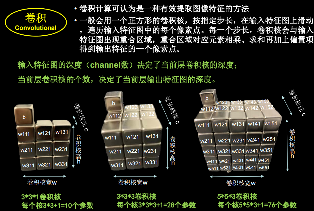
卷積計算過程

然而實際影像一般是三通道，引數會更多

先用cov進行特徵提取再進行全連線（yolo中甚至直接不用全連線，只用cov）

卷積核的channel和輸入特徵圖的channel要保持一致

輸入是三通道時

具體的計算過程

對於輸入特徵圖是三通道的

下面看一個動圖，會更好的理解

感受野

經過兩個3×3的卷積和經過一個5×5的卷積的區別是什麼？當x也就是影像邊長大於10的時候，兩個3×3的卷積比一個5×5的卷積效果要好

全零填充

如果希望卷積後輸入特徵的尺寸不變，就可以輸入特徵圖進行全0填充

計算公式

TF描述卷積層

批標準化

神經網路對零均值的資料擬合更好，但是隨著神經網路層數的增加，資料還會偏離0均值，用標準化可以把資料拉回來。一般用在卷積和啟用函式之間。

但是如果只進行上面這種簡單的標準化，資料都分佈在sigmoid函式中間的線性部分，失去了非線性化，因此又引入了兩個訓練引數，保證了網路的非線性表達力

tensorflow中是

池化

tf中的池化函式

dropout

在神經網路的訓練過程中，對於一次迭代中的某一層神經網路，先隨機選擇其中的一些神經元並將其臨時丟棄，然後再進行本次的訓練和最佳化。在下一次迭代中，繼續隨機隱藏一些神經元，直至訓練結束。由於是隨機丟棄，故而每一個批次都在訓練不同的網路。

• 然後把輸入x 透過修改後的網路前向傳播，然後把得到的損失結果透過修改的網路反向傳播。一小批（這裡的批次batch_size由自己設定）訓練樣本執行完這個過程後，在沒有被刪除的神經元上按照隨機梯度下降法更新對應的引數（w，b）
• 重複以下過程：
  1、恢復被刪掉的神經元（此時被刪除的神經元保持原樣，而沒有被刪除的神經元已經有所更新），因此每一個mini- batch都在訓練不同的網路。
  2、從隱藏層神經元中隨機選擇一個一半大小的子集臨時刪除掉（備份被刪除神經元的引數）。
  3、對一小批訓練樣本，先前向傳播然後反向傳播損失並根據隨機梯度下降法更新引數（w，b） （沒有被刪除的那一部分引數得到更新，刪除的神經元引數保持被刪除前的結果）。

卷積神經網路

Cifar10資料集

視覺化部分樣本

import tensorflow as tf
import numpy as np
import matplotlib.pyplot as plt
np.set_printoptions(threshold=np.inf)

data_cifar10=tf.keras.datasets.cifar10.load_data()
(x_train, y_train), (x_test, y_test) =data_cifar10

print(x_train.shape)
print(y_train.shape)
plt.imshow(x_train[0])
plt.show()

卷積神經網路搭建示例

一層卷積兩層全連線

import matplotlib.pyplot as plt
import tensorflow as tf
from tensorflow.keras.layers import Dense, Dropout,MaxPooling2D,Flatten,Conv2D,BatchNormalization
from tensorflow.keras import Model
import os
import numpy as np
from tensorflow_core.python.keras.layers import Activation
# np.set_printoptions(threshold=np.inf)


class Baseline(Model):
    def __init__(self):
        super(Baseline, self).__init__()
        self.conv1 = Conv2D(6, (5,5), padding='same')
        self.bn1 = BatchNormalization()
        self.a1= Activation('relu')
        self.pool1 = MaxPooling2D(pool_size=(2,2),strides=2,padding='same')
        self.d1=Dropout(0.2)

        self.flatten1 = Flatten()
        self.f1=Dense(128,activation='relu')
        self.d2=Dropout(0.2)
        self.f2=Dense(10,activation='softmax')

    def call(self,x):
        x = self.conv1(x)
        x = self.bn1(x)
        x = self.a1(x)
        x = self.pool1(x)
        x = self.d1(x)

        x = self.flatten1(x)
        x = self.f1(x)
        x =self.d2(x)
        y= self.f2(x)
        return y


(x_train, y_train), (x_test, y_test) = tf.keras.datasets.cifar10.load_data()
x_train,x_test = x_train/255.0,x_test/255.0


model = Baseline()
model.compile(optimizer=tf.keras.optimizers.Adam(lr=0.001),loss=tf.keras.losses.SparseCategoricalCrossentropy(from_logits=False)
              ,metrics=['sparse_categorical_accuracy'])

checkpoint_save_path="baseline.ckpt"
if os.path.exists(checkpoint_save_path+'.index'):
    model.load_weights(checkpoint_save_path)
    print("---------------------Loaded model---------------")

cp_callback = tf.keras.callbacks.ModelCheckpoint(filepath=checkpoint_save_path, save_weights_only=True
                                              ,save_best_only=True, verbose=1)


history=model.fit(x_train,y_train,batch_size=32, epochs=5, validation_data=(x_test, y_test)
          ,validation_freq=1,callbacks=[cp_callback])
model.summary()

file=open('weights.txt','w')
for v in model.trainable_variables:
    file.write(str(v.name)+'\n')
    file.write(str(v.shape)+'\n')
    file.write(str(v.numpy())+'\n')
file.close()

train_acc=history.history['sparse_categorical_accuracy']
val_acc=history.history['val_sparse_categorical_accuracy']
loss=history.history['loss']
val_loss=history.history['val_loss']

plt.subplot(1,2,1)
plt.plot(loss,label='train_loss')
plt.plot(val_loss,label='val_loss')
plt.title('model loss')
plt.legend()

plt.subplot(1,2,2)
plt.plot(train_acc,label='train_acc')
plt.plot(val_acc,label='val_acc')
plt.title('model acc')
plt.legend()
plt.show()

如果你是看到曹老師的課，這裡你會遇到一個問題，準確率一直在0.1，因為30和40系顯示卡不支援老版本了，解決方法看這篇文章

LeNet

import matplotlib.pyplot as plt
import tensorflow as tf
from tensorflow.keras.layers import Dense, Dropout,MaxPooling2D,Flatten,Conv2D,BatchNormalization,Activation
from tensorflow.keras import Model
import os
import numpy as np

# np.set_printoptions(threshold=np.inf)


class Baseline(Model):
    def __init__(self):
        super(Baseline, self).__init__()
        self.conv1 = Conv2D(6, (5,5), activation='sigmoid')
        self.pool1 = MaxPooling2D(pool_size=(2,2),strides=2)
        self.conv2 = Conv2D(16, (5,5), activation='sigmoid')
        self.pool2 = MaxPooling2D(pool_size=(2,2),strides=2)

        self.flatten1 = Flatten()
        self.f1=Dense(120,activation='sigmoid')
        self.f2=Dense(84,activation='sigmoid')
        self.f3=Dense(10,activation='softmax')

    def call(self,x):
        x = self.conv1(x)
        x = self.pool1(x)
        x = self.conv2(x)
        x = self.pool2(x)

        x = self.flatten1(x)
        x = self.f1(x)
        x = self.f2(x)
        y = self.f3(x)
        return y


(x_train, y_train), (x_test, y_test) = tf.keras.datasets.cifar10.load_data()
x_train,x_test = x_train/255.0,x_test/255.0


model = Baseline()
model.compile(optimizer=tf.keras.optimizers.Adam(lr=0.001),loss=tf.keras.losses.SparseCategoricalCrossentropy(from_logits=False)
              ,metrics=['sparse_categorical_accuracy'])

checkpoint_save_path="./checkpoints/lenet.ckpt"
if os.path.exists(checkpoint_save_path+'.index'):
    model.load_weights(checkpoint_save_path)
    print("---------------------Loaded model---------------")

cp_callback = tf.keras.callbacks.ModelCheckpoint(filepath=checkpoint_save_path, save_weights_only=True
                                              ,save_best_only=True, verbose=1)


history=model.fit(x_train,y_train,batch_size=32, epochs=5, validation_data=(x_test, y_test)
          ,validation_freq=1,callbacks=[cp_callback])
model.summary()

file=open('./checkpoints/weights_lenet.txt','w')
for v in model.trainable_variables:
    file.write(str(v.name)+'\n')
    file.write(str(v.shape)+'\n')
    file.write(str(v.numpy())+'\n')
file.close()

train_acc=history.history['sparse_categorical_accuracy']
val_acc=history.history['val_sparse_categorical_accuracy']
loss=history.history['loss']
val_loss=history.history['val_loss']

plt.subplot(1,2,1)
plt.plot(loss,label='train_loss')
plt.plot(val_loss,label='val_loss')
plt.title('model loss')
plt.legend()

plt.subplot(1,2,2)
plt.plot(train_acc,label='train_acc')
plt.plot(val_acc,label='val_acc')
plt.title('model acc')
plt.legend()
plt.show()

AlexNet

共8層

網路架構

import matplotlib.pyplot as plt
import tensorflow as tf
from tensorflow.keras.layers import Dense, Dropout,MaxPooling2D,Flatten,Conv2D,BatchNormalization,Activation,Flatten
from tensorflow.keras import Model
import os
import numpy as np

# np.set_printoptions(threshold=np.inf)


class AlexNet(Model):
    def __init__(self):
        super(AlexNet, self).__init__()
        self.conv1 = Conv2D(96, kernel_size=(3,3), padding='valid')
        self.bn1 = BatchNormalization()
        self.a1= Activation('relu')
        self.pool1 = MaxPooling2D(pool_size=(3,3),strides=2)

        self.conv2 = Conv2D(256, (3,3), padding='valid')
        self.bn2 = BatchNormalization()
        self.a2= Activation('relu')
        self.pool2 = MaxPooling2D(pool_size=(3,3),strides=2)

        self.conv3 = Conv2D(384, (3,3), padding='same',activation='relu')

        self.conv4 = Conv2D(384, (3,3), padding='same',activation='relu')

        self.conv5 = Conv2D(256, (3,3), padding='same',activation='relu')
        self.pool5 = MaxPooling2D(pool_size=(3,3),strides=2)

        self.flatten1 = Flatten()
        self.f1=Dense(2048,activation='relu')
        self.d1=Dropout(0.5)
        self.f2=Dense(2048,activation='relu')
        self.d2=Dropout(0.5)
        self.f3=Dense(10,activation='softmax')

    def call(self,x):
        x=self.conv1(x)
        x=self.bn1(x)
        x=self.a1(x)
        x=self.pool1(x)

        x=self.conv2(x)
        x=self.bn2(x)
        x=self.a2(x)
        x=self.pool2(x)

        x=self.conv3(x)

        x=self.conv4(x)

        x=self.conv5(x)
        x=self.pool5(x)

        x=self.flatten1(x)
        x=self.f1(x)
        x=self.d1(x)
        x=self.f2(x)
        x=self.d2(x)
        y=self.f3(x)
        return y


(x_train, y_train), (x_test, y_test) = tf.keras.datasets.cifar10.load_data()
x_train,x_test = x_train/255.0,x_test/255.0


model = AlexNet()
model.compile(optimizer='Adam',loss=tf.keras.losses.SparseCategoricalCrossentropy(from_logits=False)
              ,metrics=['sparse_categorical_accuracy'])

checkpoint_save_path="./checkpoints/Alex.ckpt"
if os.path.exists(checkpoint_save_path+'.index'):
    model.load_weights(checkpoint_save_path)
    print("---------------------Loaded model---------------")

cp_callback = tf.keras.callbacks.ModelCheckpoint(filepath=checkpoint_save_path, save_weights_only=True
                                              ,save_best_only=True, verbose=1)


history=model.fit(x_train,y_train,batch_size=32, epochs=5, validation_data=(x_test, y_test)
          ,validation_freq=1,callbacks=[cp_callback])
model.summary()

file=open('./checkpoints/weights_alex.txt','w')
for v in model.trainable_variables:
    file.write(str(v.name)+'\n')
    file.write(str(v.shape)+'\n')
    file.write(str(v.numpy())+'\n')
file.close()

train_acc=history.history['sparse_categorical_accuracy']
val_acc=history.history['val_sparse_categorical_accuracy']
loss=history.history['loss']
val_loss=history.history['val_loss']

plt.subplot(1,2,1)
plt.plot(loss,label='train_loss')
plt.plot(val_loss,label='val_loss')
plt.title('model loss')
plt.legend()

plt.subplot(1,2,2)
plt.plot(train_acc,label='train_acc')
plt.plot(val_acc,label='val_acc')
plt.title('model acc')
plt.legend()
plt.show()

VGGNet

import matplotlib.pyplot as plt
import tensorflow as tf
from tensorflow.keras.layers import Dense, Dropout,MaxPooling2D,Flatten,Conv2D,BatchNormalization,Activation,Flatten
from tensorflow.keras import Model
import os
import numpy as np

# np.set_printoptions(threshold=np.inf)


class VGG16(Model):
    def __init__(self):
        super(VGG16, self).__init__()
        self.conv1 = Conv2D(64, (3, 3),padding='same')
        self.bn1 = BatchNormalization()
        self.a1= Activation('relu')

        self.conv2 = Conv2D(64, (3, 3),padding='same')
        self.bn2 = BatchNormalization()
        self.a2= Activation('relu')
        self.pool2 = MaxPooling2D((2, 2), strides=2,padding='same')
        self.d2=Dropout(0.2)

        self.conv3 = Conv2D(128, (3, 3),padding='same')
        self.bn3= BatchNormalization()
        self.a3= Activation('relu')

        self.conv4 = Conv2D(128, (3, 3),padding='same')
        self.bn4=BatchNormalization()
        self.a4= Activation('relu')
        self.p4= MaxPooling2D((2, 2), strides=2,padding='same')
        self.d4= Dropout(0.2)

        self.conv5 = Conv2D(256, (3, 3),padding='same')
        self.bn5=BatchNormalization()
        self.a5= Activation('relu')

        self.conv6= Conv2D(256, (3, 3),padding='same')
        self.bn6= BatchNormalization()
        self.a6= Activation('relu')

        self.conv7= Conv2D(256, (3, 3),padding='same')
        self.bn7= BatchNormalization()
        self.a7= Activation('relu')
        self.p7= MaxPooling2D((2, 2), strides=2,padding='same')
        self.d7= Dropout(0.2)

        self.conv8= Conv2D(512, (3, 3),padding='same')
        self.bn8=BatchNormalization()
        self.a8= Activation('relu')

        self.conv9= Conv2D(512, (3, 3),padding='same')
        self.bn9= BatchNormalization()
        self.a9= Activation('relu')

        self.conv10= Conv2D(512, (3, 3),padding='same')
        self.bn10= BatchNormalization()
        self.a10= Activation('relu')
        self.p10= MaxPooling2D((2, 2), strides=2,padding='same')
        self.d10= Dropout(0.2)

        self.conv11= Conv2D(512, (3, 3),padding='same')
        self.bn11= BatchNormalization()
        self.a11= Activation('relu')

        self.conv12= Conv2D(512, (3, 3),padding='same')
        self.bn12= BatchNormalization()
        self.a12= Activation('relu')

        self.conv13= Conv2D(512, (3, 3),padding='same')
        self.bn13= BatchNormalization()
        self.a13= Activation('relu')
        self.p13= MaxPooling2D((2, 2), strides=2,padding='same')
        self.d13= Dropout(0.2)

        self.flatten= Flatten()
        self.fc14= Dense(512,activation='relu')
        self.d14=Dropout(0.2)
        self.fc15= Dense(512,activation='relu')
        self.d15= Dropout(0.2)
        self.fc16=Dense(10,activation='softmax')


    def call(self,x):
        x = self.conv1(x)
        x=self.bn1(x)
        x=self.a1(x)

        x=self.conv2(x)
        x=self.bn2(x)
        x=self.a2(x)
        x=self.pool2(x)
        x=self.d2(x)

        x=self.conv3(x)
        x=self.bn3(x)
        x=self.a3(x)

        x=self.conv4(x)
        x=self.bn4(x)
        x=self.a4(x)
        x=self.p4(x)
        x=self.d4(x)

        x=self.conv5(x)
        x=self.bn5(x)
        x=self.a5(x)

        x=self.conv6(x)
        x=self.bn6(x)
        x=self.a6(x)

        x=self.conv7(x)
        x=self.bn7(x)
        x=self.a7(x)
        x=self.p7(x)
        x=self.d7(x)

        x=self.conv8(x)
        x=self.bn8(x)
        x=self.a8(x)

        x=self.conv9(x)
        x=self.bn9(x)
        x=self.a9(x)

        x=self.conv10(x)
        x=self.bn10(x)
        x=self.a10(x)
        x=self.p10(x)
        x=self.d10(x)

        x=self.conv11(x)
        x=self.bn11(x)
        x=self.a11(x)

        x=self.conv12(x)
        x=self.bn12(x)
        x=self.a12(x)

        x=self.conv13(x)
        x=self.bn13(x)
        x=self.a13(x)
        x=self.p13(x)
        x=self.d13(x)

        x=self.flatten(x)
        x=self.fc14(x)
        x=self.fc15(x)
        y=self.fc16(x)
        return y


(x_train, y_train), (x_test, y_test) = tf.keras.datasets.cifar10.load_data()
x_train,x_test = x_train/255.0,x_test/255.0


model = VGG16()
model.compile(optimizer='Adam',loss=tf.keras.losses.SparseCategoricalCrossentropy(from_logits=False)
              ,metrics=['sparse_categorical_accuracy'])

checkpoint_save_path="./checkpoints/VGG16.ckpt"
if os.path.exists(checkpoint_save_path+'.index'):
    model.load_weights(checkpoint_save_path)
    print("---------------------Loaded model---------------")

cp_callback = tf.keras.callbacks.ModelCheckpoint(filepath=checkpoint_save_path, save_weights_only=True
                                              ,save_best_only=True, verbose=1)


history=model.fit(x_train,y_train,batch_size=32, epochs=5, validation_data=(x_test, y_test)
          ,validation_freq=1,callbacks=[cp_callback])
model.summary()

file=open('./checkpoints/weights_VGG16.txt','w')
for v in model.trainable_variables:
    file.write(str(v.name)+'\n')
    file.write(str(v.shape)+'\n')
    file.write(str(v.numpy())+'\n')
file.close()

train_acc=history.history['sparse_categorical_accuracy']
val_acc=history.history['val_sparse_categorical_accuracy']
loss=history.history['loss']
val_loss=history.history['val_loss']

plt.subplot(1,2,1)
plt.plot(loss,label='train_loss')
plt.plot(val_loss,label='val_loss')
plt.title('model loss')
plt.legend()

plt.subplot(1,2,2)
plt.plot(train_acc,label='train_acc')
plt.plot(val_acc,label='val_acc')
plt.title('model acc')
plt.legend()
plt.show()

Inception

引入Inception結構塊，在同一層網路內使用不同尺寸的卷積核，提升了模型感知力；使用了批標準化，緩解了梯度消失。

核心是它的基本單元Inception結構塊，無論是GoogLeNet（Inception v1），還是InceptionNet的後續版本，比如v2/v3/v4，

都是基於Inception結構塊搭建的網路。Inception結構塊在同一層網路中使用了多個尺寸的卷積核，可以提取不同尺寸的特徵。

透過1×1卷積核作用到輸入特徵圖的每個畫素點，透過設定少於輸入特徵圖深度的1*1卷積核個數，減少了輸出特徵圖深度，起到

了降維的作用，減少了引數量和計算量。

Inception有四個分支，具體結構見上圖右上角

裡面有很多重複的程式碼，編寫ConvBNRelu類，增加程式碼可讀性。

有了Inception塊後，就能搭建精簡版本的InceptionNet

網路共有10層，第一次是一個3×3的conv，然後是4個Inception結構塊順序相連，每兩個Inception結構塊組成一個block每個block中的第一個Inception結構塊卷積步長是2，第二個Inception結構塊卷積步長是1，這使得第一個Inception結構塊輸出特徵圖尺寸減半，因此把輸出特徵圖深度加深，儘可能保證特徵抽取中資訊的承載量一致。

block_0設定的卷積核個數是16，經過了四個分支，輸出的深度為4 * 16=64。block_1卷積核個數是block_0通的兩倍（self.out_channels * = 2），是32，同樣經過了四個分支，輸出深度是4*32=128.這128個通道的資料會被送入平均池化，送入10個分類的全連線

首先我們簡單理解全域性平均池化操作。之前我們需要把特徵圖展開然後進行全連線，而現在，我們直接沒有了這一步。
如果有一批特徵圖，其尺寸為 [ B, C, H, W], 我們經過全域性平均池化之後，尺寸變為[B, C, 1, 1]。
也就是說，全域性平均池化其實就是對每一個通道圖所有畫素值求平均值，然後得到一個新的1 * 1的通道圖。

由於網路規模比較大，把batch_size調整到1024，讓訓練時一次喂入神經網路的資料量多一些，以充分發揮顯示卡的效能，提高訓練速度

一般讓顯示卡達到70-80%的負荷比較合理。注意：資料量大的時候可以調大batchsize，資料量小的時候batchsize不要調太大，因為資料量小的時候，如果batchsize小，那麼一個epoch會有很多batchsize，每一個batchsize都會進行梯度更新。

import matplotlib.pyplot as plt
import tensorflow as tf
from tensorflow.keras.layers import Dense, Dropout,MaxPooling2D,Flatten,Conv2D,BatchNormalization,\
    Activation,Flatten,GlobalAveragePooling2D
from tensorflow.keras import Model, Sequential
import os
import numpy as np

# np.set_printoptions(threshold=np.inf)


class ConvBNRelu(Model):
    def __init__(self,filters,kernel_size,stride=1):
        super(ConvBNRelu, self).__init__()
        self.model = Sequential([
            Conv2D(filters, kernel_size,strides=stride, padding='same'),
            BatchNormalization(),
            Activation('relu'),
        ])

    def call(self,x):
        y=self.model(x,training=False)
        return y


class Inception(Model):
    def __init__(self,init_ch,stride):
        super(Inception, self).__init__()
        self.c1=ConvBNRelu(init_ch,1,stride=stride)  # 方便下面Inception10控制特徵圖的size
        self.c2_1=ConvBNRelu(init_ch,1,stride=stride) #
        self.c2_2=ConvBNRelu(init_ch,3)
        self.c3_1=ConvBNRelu(init_ch,1,stride=stride) #
        self.c3_2=ConvBNRelu(init_ch,5)
        self.c4_1=MaxPooling2D((3,3),strides=(1,1),padding='same')
        self.c4_2=ConvBNRelu(init_ch,1,stride=stride)  #

    def call(self,x):
        x1=self.c1(x)  # x=self.c1(x)
        x2=self.c2_1(x)
        x2=self.c2_2(x2)
        x3=self.c3_1(x)
        x3=self.c3_2(x3)
        x4=self.c4_1(x)
        x4=self.c4_2(x4)
        y=tf.concat([x1,x2,x3,x4],axis=3)
        return y


class Inception10(Model):
    def __init__(self,num_classes,block_n,init_ch=16):
        super(Inception10,self).__init__()
        self.channel=init_ch   # 卷積核個數
        self.blocks=Sequential()
        self.c1=ConvBNRelu(16,3)  # 最開頭的那一層
        for i in range(block_n):
            for j in range(2):
                if j%2==0:
                    block=Inception(self.channel,stride=2)
                else:
                    block=Inception(self.channel,stride=1)
                self.blocks.add(block)   # 
            self.channel*=2     # stride=2會使特徵圖size變小，透過增加channnel來表示更多資訊
        self.pool=GlobalAveragePooling2D()
        self.dense=Dense(num_classes,activation='softmax')

    def call(self,x):
        x=self.c1(x)
        x = self.blocks(x)
        x = self.pool(x)
        x = self.dense(x)
        return x

(x_train, y_train), (x_test, y_test) = tf.keras.datasets.cifar10.load_data()
x_train,x_test = x_train/255.0,x_test/255.0


model = Inception10(10,block_n=2)
model.compile(optimizer='Adam',loss=tf.keras.losses.SparseCategoricalCrossentropy(from_logits=False)
              ,metrics=['sparse_categorical_accuracy'])

checkpoint_save_path="./checkpoints/Inception10_gai2.ckpt"
if os.path.exists(checkpoint_save_path+'.index'):
    model.load_weights(checkpoint_save_path)
    print("---------------------Loaded model---------------")

cp_callback = tf.keras.callbacks.ModelCheckpoint(filepath=checkpoint_save_path, save_weights_only=True
                                              ,save_best_only=True, verbose=1)


history=model.fit(x_train,y_train,batch_size=32, epochs=5, validation_data=(x_test, y_test)
          ,validation_freq=1,callbacks=[cp_callback])
model.summary()

file=open('./checkpoints/weights_Inception10_gai2.txt','w')
for v in model.trainable_variables:
    file.write(str(v.name)+'\n')
    file.write(str(v.shape)+'\n')
    file.write(str(v.numpy())+'\n')
file.close()

train_acc=history.history['sparse_categorical_accuracy']
val_acc=history.history['val_sparse_categorical_accuracy']
loss=history.history['loss']
val_loss=history.history['val_loss']

plt.subplot(1,2,1)
plt.plot(loss,label='train_loss')
plt.plot(val_loss,label='val_loss')
plt.title('model loss')
plt.legend()

plt.subplot(1,2,2)
plt.plot(train_acc,label='train_acc')
plt.plot(val_acc,label='val_acc')
plt.title('model acc')
plt.legend()
plt.show()

ResNet

提出了層間殘差跳連，引入了前方資訊，緩解梯度消失，使神經網路層數增加成為可能

單純堆疊神經網路層數會使神經網路模型退化，以至於後邊的特徵丟失了前邊特徵的原本模樣

用了一根跳連線，將前邊的特徵直接接到了後邊，使輸出結果H(x)包含了堆疊卷積的非線性輸出F(x)，和跳過這兩層堆疊卷積、直接連線過來的恆等對映x，讓它們對應元素相加。這一操作有效緩解了神經網路模型堆疊導致的退化，使得神經網路可以向著更深層級發展。

ResNet塊中有兩種情況，一種是用下圖實線表示，兩層堆疊卷積沒有改變特徵圖的維度，即特徵圖的個數、高、寬和深度都相同，可以直接將F(x)與x相加。另一種情況用虛線表示，兩層堆疊卷積改變了特徵圖的維度，需要藉助1*1的卷積來調整x的維度，使W(x)與F(x)維度一致

如果堆疊卷積層前後維度不同，residual_path=1，使用1*1卷積操作調整輸入特徵圖inputs的尺寸或深度後，將堆疊卷積輸出特徵y和if語句計算出的residual相加，過啟用，輸出如果堆疊卷積層前後維度相同，直接將堆疊卷積輸出特徵y和輸入特徵圖inputs相加，過啟用，輸出。下面的黃色框就是一個block，橘黃色框裡有兩種不同情況的block

ResNet18：8個ResNet塊,每一個ResNet塊有兩層卷積，一共是18層網路。為了加速模型收斂，把batch_size調到128

import matplotlib.pyplot as plt
import tensorflow as tf
from tensorflow.keras.layers import Dense, Dropout,MaxPooling2D,Flatten,Conv2D,BatchNormalization,\
    Activation,Flatten,GlobalAveragePooling2D
from tensorflow.keras import Model, Sequential
import os
import numpy as np

# np.set_printoptions(threshold=np.inf)


class ResNetBlock(Model):
    def __init__(self, filters, stride,residual):
        super(ResNetBlock, self).__init__()
        self.filters = filters
        self.strides = stride
        self.residual = residual

        self.conv1 = Conv2D(self.filters, 3, strides=self.strides,padding='same',use_bias=False)
        self.bn1 = BatchNormalization()
        self.a1= Activation('relu')

        self.conv2 = Conv2D(self.filters, 3, strides=1,padding='same',use_bias=False)
        self.bn2 = BatchNormalization()

        if residual:
            self.conv3 = Conv2D(self.filters, 1, strides=self.strides,padding='same',use_bias=False)
            self.bn3 = BatchNormalization()
        self.a2 = Activation('relu')

    def call(self, inputs,*args, **kwargs):
        resi = inputs
        x = self.conv1(inputs)
        x = self.bn1(x)
        x = self.a1(x)

        x = self.conv2(x)
        x = self.bn2(x)

        if self.residual:
            y=self.conv3(inputs)    #
            y=self.bn3(y)
            resi=y

        return self.a2(x+resi)


class ResNet18(Model):
    def __init__(self,block_list,init_channels,num_classes):
        super(ResNet18, self).__init__()
        self.conv1 = Conv2D(64,3,strides=1,padding='same',use_bias=False)
        self.bn1 = BatchNormalization()
        self.a1 = Activation('relu')

        self.ll=len(block_list)
        self.blocks=Sequential()
        for block_i in range(self.ll):
            for layer in range(block_list[block_i]):
                if block_i !=0 and layer==0:
                    self.blocks.add(ResNetBlock(init_channels,2,residual=True))
                else:
                    self.blocks.add(ResNetBlock(init_channels,1,residual=False))
            init_channels=init_channels*2
        self.p1=GlobalAveragePooling2D()
        self.f1=Dense(num_classes,activation='softmax',kernel_regularizer=tf.keras.regularizers.l2())

    def call(self, inputs,*args, **kwargs):
        x = self.conv1(inputs)
        x=self.bn1(x)
        x = self.a1(x)
        x=self.blocks(x)
        x=self.p1(x)
        x=self.f1(x)
        return x





(x_train, y_train), (x_test, y_test) = tf.keras.datasets.cifar10.load_data()
x_train,x_test = x_train/255.0,x_test/255.0


model = ResNet18([2,2,2,2],64,num_classes=10)
model.compile(optimizer='Adam',loss=tf.keras.losses.SparseCategoricalCrossentropy(from_logits=False)
              ,metrics=['sparse_categorical_accuracy'])

checkpoint_save_path="./checkpoints/ResNet18.ckpt"
if os.path.exists(checkpoint_save_path+'.index'):
    model.load_weights(checkpoint_save_path)
    print("---------------------Loaded model---------------")

cp_callback = tf.keras.callbacks.ModelCheckpoint(filepath=checkpoint_save_path, save_weights_only=True
                                              ,save_best_only=True, verbose=1)


history=model.fit(x_train,y_train,batch_size=32, epochs=5, validation_data=(x_test, y_test)
          ,validation_freq=1,callbacks=[cp_callback])
model.summary()

file=open('./checkpoints/weights_ResNet18txt','w')
for v in model.trainable_variables:
    file.write(str(v.name)+'\n')
    file.write(str(v.shape)+'\n')
    file.write(str(v.numpy())+'\n')
file.close()

train_acc=history.history['sparse_categorical_accuracy']
val_acc=history.history['val_sparse_categorical_accuracy']
loss=history.history['loss']
val_loss=history.history['val_loss']

plt.subplot(1,2,1)
plt.plot(loss,label='train_loss')
plt.plot(val_loss,label='val_loss')
plt.title('model loss')
plt.legend()

plt.subplot(1,2,2)
plt.plot(train_acc,label='train_acc')
plt.plot(val_acc,label='val_acc')
plt.title('model acc')
plt.legend()
plt.show()

可以比較一下這幾個模型在cifar10上的表現，epoch=5，batchsize=32

Model	train_acc	val_acc
baseline	0.5469	0.4969
LeNet	0.4435	0.4407
AlexNet	0.6545	0.5186
VGGNet	0.7525	0.7039
Inception10	0.7927	0.7444
ResNet18	0.8688	0.7946

經典卷積網路小結

class6

迴圈核

有些資料是和時間序列相關的，是可以根據上午預測出下文的

給你一段話，魚離不開_,你可能下意識會說水，因為你記住了前面的四個，可以推出大機率是水

輸入\(x_t\)維度和輸出\(y_t\)的維度，以及迴圈核的個數確定，三個引數矩陣的維度也就確定了

每一個迴圈核構成一個迴圈計算層

TF描述迴圈計算層

return_sequences設為False，True的區別如下（布林。是返回輸出序列中的最後一個輸出，還是返回完整序列。預設值：False。）

對輸入的樣本維度有要求

迴圈計算過程 I

記憶體的個數為3，\(W_{hx},W_{hh},W_{hy}\)是訓練好的引數。過tanh啟用函式後得到當前時刻的狀態資訊ht

記憶體儲存的狀態資訊被重新整理為[-0.9,0.8,0.7],然後輸出yt是把提取到的時間資訊，透過全連線進行識別預測的過程，是整個網路的輸出層

模型認為有91%的機率輸出c。下面看一下程式碼實現

字母預測onehot_1pre1

用RNN實現輸入一個字母，預測下一個字母（One hot 編碼）

SimpleRNN(3),  # 這裡可以自行調節記憶體個數
Dense(5, activation='softmax')  # 一層全連線，實現輸出層yt的計算，由於要對映到獨立熱編碼，找到最大機率字母，所以=5

程式碼

迴圈計算過程2

前面是輸入是一個字母，預測下一個字母。現在感受一下把迴圈核按時間步展開，連續輸入多個字母預測下一個字母。仍然使用三個記憶體，初始為0，用一套訓練好的引數矩陣，帶你感受迴圈計算的前向傳播

輸入b更新記憶體

這四個時間步中所用到的引數矩陣，Wxh和bh是完全相同的。輸出預測透過全連線完成

百分之70機率是a，預測正確。

字母預測onehot_4pre1

需要修改的地方不多

程式碼如下

import os

import tensorflow as tf
from tensorflow.keras import Sequential
from tensorflow.keras.layers import SimpleRNN, Dense, Dropout
import numpy as np
import matplotlib.pyplot as plt


inputs_word='abcde'
word_id={'a':0,'b':1,'c':2,'d':3,'e':4}
id_onehot={0:[1.,0.,0.,0.,0.],1:[0.,1.,0.,0.,0.],2:[0.,0.,1.,0.,0.],3:[0.,0.,0.,1.,0.],4:[0.,0.,0.,0.,1.]}

x_train=[
    [id_onehot[word_id['a']],id_onehot[word_id['b']],id_onehot[word_id['c']],id_onehot[word_id['d']]],
    [id_onehot[word_id['b']],id_onehot[word_id['c']],id_onehot[word_id['d']],id_onehot[word_id['e']]],
    [id_onehot[word_id['c']],id_onehot[word_id['d']],id_onehot[word_id['e']],id_onehot[word_id['a']]],
    [id_onehot[word_id['d']],id_onehot[word_id['e']],id_onehot[word_id['a']],id_onehot[word_id['b']]],
    [id_onehot[word_id['e']],id_onehot[word_id['a']],id_onehot[word_id['b']],id_onehot[word_id['c']]]
]
# y_train=[id_onehot[word_id['e']],id_onehot[word_id['a']],id_onehot[word_id['b']],id_onehot[word_id['c']],id_onehot[word_id['d']]] #錯的
y_train=[word_id['e'],word_id['a'],word_id['b'],word_id['c'],word_id['d']]
# x_train=np.array(x_train)
# y_train=np.array(y_train)
# print(x_train.shape)  # (4, 4, 5)
# print(y_train.shape)  # (4, 5)
np.random.seed(7)
np.random.shuffle(x_train)
np.random.seed(7)
np.random.shuffle(y_train)
tf.random.set_seed(7)


x_train=np.reshape(x_train,[len(x_train),4,5])
y_train=np.array(y_train)


model=Sequential([
    SimpleRNN(3),
    Dense(units=5,activation='softmax')
])

model.compile(tf.keras.optimizers.Adam(0.01),loss=tf.keras.losses.SparseCategoricalCrossentropy(from_logits=False),
              metrics=['sparse_categorical_accuracy'])

checkpoint_path="./checkpoint/rnn_ont4pre1.ckpt"
if os.path.exists(checkpoint_path+'.index'):
    print('---------------------load  model-------------------------')
    model.load_weights(checkpoint_path)

cp_callback = tf.keras.callbacks.ModelCheckpoint(checkpoint_path,monitor='loss',
                                                 save_best_only=True,save_weights_only=True)

history=model.fit(x_train,y_train,batch_size=32,epochs=100,callbacks=[cp_callback])
model.summary()

acc = history.history['sparse_categorical_accuracy']
loss = history.history['loss']

plt.subplot(1, 2, 1)
plt.plot(acc, label='Training Accuracy')
plt.title('Training Accuracy')
plt.legend()

plt.subplot(1, 2, 2)
plt.plot(loss, label='Training Loss')
plt.title('Training Loss')
plt.legend()
plt.show()

input_s=int(input("Enter the number "))
for i in range(input_s):
    x=input('輸入一串字串，長度為4')
    x_pre=[id_onehot[word_id[a]] for a in x]
    x_pre=np.reshape(x_pre,(1,4,5))
    y_pred=model.predict(x_pre)
    y_pred=np.argmax(y_pred,axis=1)
    y=int(y_pred)
    print(inputs_word[y])

Embedding編碼

用RNN實現輸入一個字母，預測下一個字母（Embedding 編碼）

全部程式碼如下

import os

import tensorflow as tf
from tensorflow.keras import Sequential
from tensorflow.keras.layers import SimpleRNN, Dense, Dropout,Embedding
import numpy as np
import matplotlib.pyplot as plt


inputs_word='abcde'
word_id={'a':0,'b':1,'c':2,'d':3,'e':4}

x_train=[word_id['a'],word_id['b'],word_id['c'],word_id['d'],word_id['e']]
y_train=[word_id['b'],word_id['c'],word_id['d'],word_id['e'],word_id['a']]

np.random.seed(7)
np.random.shuffle(x_train)
np.random.seed(7)
np.random.shuffle(y_train)
tf.random.set_seed(7)


x_train=np.reshape(x_train,[len(x_train),1])
y_train=np.array(y_train)


model=Sequential([
    Embedding(5,3),   # (5,2),(5,5),(5,4)  第一個數是字典長度，即輸入資料最大下標+1。第二個數可以隨意，表示嵌入的維度
    SimpleRNN(3),
    Dense(units=5,activation='softmax')
])

model.compile(tf.keras.optimizers.Adam(0.01),loss=tf.keras.losses.SparseCategoricalCrossentropy(from_logits=False),
              metrics=['sparse_categorical_accuracy'])

checkpoint_path="./checkpoint/rnn_Embed1pre1.ckpt"
if os.path.exists(checkpoint_path+'.index'):
    print('---------------------load  model-------------------------')
    model.load_weights(checkpoint_path)

cp_callback = tf.keras.callbacks.ModelCheckpoint(checkpoint_path,monitor='loss',
                                                 save_best_only=True,save_weights_only=True)

history=model.fit(x_train,y_train,batch_size=32,epochs=100,callbacks=[cp_callback])
model.summary()

acc = history.history['sparse_categorical_accuracy']
loss = history.history['loss']

plt.subplot(1, 2, 1)
plt.plot(acc, label='Training Accuracy')
plt.title('Training Accuracy')
plt.legend()

plt.subplot(1, 2, 2)
plt.plot(loss, label='Training Loss')
plt.title('Training Loss')
plt.legend()
plt.show()

input_s=int(input("Enter the number "))
for i in range(input_s):
    al=input('輸入一個字串')
    x=word_id[al]
    x=np.reshape(x,(1,1))
    y=model.predict(x)
    y=np.argmax(y,axis=1)
    y=int(y)
    print(al+'--->'+inputs_word[y])

用Embedding預測4pre1

用RNN實現輸入連續四個字母，預測下一個字母（Embedding 編碼）

增加了資料範圍

程式碼如下

import os

import tensorflow as tf
from tensorflow.keras import Sequential
from tensorflow.keras.layers import SimpleRNN, Dense, Dropout,Embedding
import numpy as np
import matplotlib.pyplot as plt


input_word = "abcdefghijklmnopqrstuvwxyz"
w_to_id = {'a': 0, 'b': 1, 'c': 2, 'd': 3, 'e': 4,
           'f': 5, 'g': 6, 'h': 7, 'i': 8, 'j': 9,
           'k': 10, 'l': 11, 'm': 12, 'n': 13, 'o': 14,
           'p': 15, 'q': 16, 'r': 17, 's': 18, 't': 19,
           'u': 20, 'v': 21, 'w': 22, 'x': 23, 'y': 24, 'z': 25}  # 單詞對映到數值id的詞典

training_set_scaled = [0, 1, 2, 3, 4, 5, 6, 7, 8, 9, 10,
                       11, 12, 13, 14, 15, 16, 17, 18, 19, 20,
                       21, 22, 23, 24, 25]

x_train=[]
y_train=[]
for i in range(4,26):
    x_train.append(training_set_scaled[i-4:i])
    y_train.append(training_set_scaled[i])

np.random.seed(7)
np.random.shuffle(x_train)
np.random.seed(7)
np.random.shuffle(y_train)
tf.random.set_seed(7)

x_train=np.reshape(x_train,[len(x_train),4])
y_train=np.array(y_train)


model=Sequential([
    Embedding(26,3),
    SimpleRNN(10),
    Dense(units=26,activation='softmax')
])

model.compile(tf.keras.optimizers.Adam(0.01),loss=tf.keras.losses.SparseCategoricalCrossentropy(from_logits=False),
              metrics=['sparse_categorical_accuracy'])

checkpoint_path="./checkpoint/rnn_Embed4pre4.ckpt"
if os.path.exists(checkpoint_path+'.index'):
    print('---------------------load  model-------------------------')
    model.load_weights(checkpoint_path)

cp_callback = tf.keras.callbacks.ModelCheckpoint(checkpoint_path,monitor='loss',
                                                 save_best_only=True,save_weights_only=True)

history=model.fit(x_train,y_train,batch_size=32,epochs=100,callbacks=[cp_callback])
model.summary()

acc = history.history['sparse_categorical_accuracy']
loss = history.history['loss']

plt.subplot(1, 2, 1)
plt.plot(acc, label='Training Accuracy')
plt.title('Training Accuracy')
plt.legend()

plt.subplot(1, 2, 2)
plt.plot(loss, label='Training Loss')
plt.title('Training Loss')
plt.legend()
plt.show()

input_s=int(input("Enter the number "))
for i in range(input_s):
    x=input('輸入一串字串，長度為4')
    x_pre=[w_to_id[a] for a in x]
    x_pre=np.reshape(x_pre,(1,4))
    y_pred=model.predict(x_pre)
    y_pred=np.argmax(y_pred,axis=1)
    y=int(y_pred)
    print(input_word[y])

RNN實現股票預測

Minmax Scaler不能處理特徵只有一維的資料，需要.reshape(-1,1),檔案下載

import os
from sklearn.metrics import mean_squared_error, mean_absolute_error
import tensorflow as tf
import numpy as np
import matplotlib.pyplot as plt
import pandas as pd
from sklearn.preprocessing import MinMaxScaler
from tensorflow.keras.layers import Dense, Dropout,SimpleRNN
from tensorflow.keras import Sequential
import math

df=pd.read_csv('./class6/SH600519.csv')

x_train=df.iloc[:2426-300,2].values.reshape(-1,1)
x_test=df.iloc[2426-300:,2].values.reshape(-1,1)

scaler=MinMaxScaler(feature_range=(0,1))
x_train=scaler.fit_transform(x_train)
x_test=scaler.transform(x_test)

x_data_train=[]
y_data_train=[]

for i in range(60,len(x_train)):
    ss=x_train[i-60:i,0]
    # sss=x_train[i-60:i]
    x_data_train.append(ss)
    xx=x_train[i,0]
    y_data_train.append(xx)

x_data_test=[]
y_data_test=[]
for i in range(60,len(x_test)):
    ss=x_test[i-60:i,0]
    x_data_test.append(ss)
    xx=x_test[i,0]
    y_data_test.append(xx)


np.random.seed(33)
np.random.shuffle(x_data_train)
np.random.seed(33)
np.random.shuffle(y_data_train)

x_data_train,y_data_train=np.array(x_data_train),np.array(y_data_train)
x_data_test,y_data_test=np.array(x_data_test),np.array(y_data_test)
x_data_train=np.reshape(x_data_train,(len(x_data_train),60,1))
x_data_test=np.reshape(x_data_test,(len(x_data_test),60,1))

model=Sequential(
    [
        SimpleRNN(units=80,return_sequences=True),
        Dropout(0.2),
        SimpleRNN(units=100),
        Dropout(0.2),
        Dense(1)
    ]
)

model.compile(optimizer='adam',loss='mean_squared_error')

checkpoint_path='./checkpoint/rnn_maotai.ckpt'
if os.path.exists(checkpoint_path+'.index'):
    print('------------------load model -----------------')
    model.load_weights(checkpoint_path)

cp_callback = tf.keras.callbacks.ModelCheckpoint(checkpoint_path,save_best_only=True,save_weights_only=True)

history=model.fit(x_data_train,y_data_train,epochs=50,callbacks=[cp_callback],validation_data=(x_data_test,y_data_test),
                  batch_size=64,validation_freq=1)
model.summary()


loss = history.history['loss']
val_loss = history.history['val_loss']
plt.plot(loss, label='Training Loss')
plt.plot(val_loss, label='Validation Loss')
plt.title('Training and Validation Loss')
plt.legend()
plt.show()

y_pred = model.predict(x_data_test)
y_pred = scaler.inverse_transform(y_pred)

y_true=scaler.inverse_transform(x_test[60:])

plt.plot(y_true, color='red', label='MaoTai Stock Price')
plt.plot(y_pred, color='blue', label='Predicted MaoTai Stock Price')
plt.title('MaoTai Stock Price Prediction')
plt.xlabel('Time')
plt.ylabel('MaoTai Stock Price')
plt.legend()
plt.show()

mse = mean_squared_error(y_pred, y_true)
rmse = math.sqrt(mean_squared_error(y_pred, y_true))
mae = mean_absolute_error(y_pred, y_true)
print('均方誤差: %.6f' % mse)
print('均方根誤差: %.6f' % rmse)
print('平均絕對誤差: %.6f' % mae)

使用LSTM實現股票預測

當序列長度過長時，RNN的表現並不理想，能不能讓網路記憶一個很長序列

tf中LSTM程式碼如下

需要改動的只有model裡面，其他和上一個程式碼完全相同

import os
from sklearn.metrics import mean_squared_error, mean_absolute_error
import tensorflow as tf
import numpy as np
import matplotlib.pyplot as plt
import pandas as pd
from sklearn.preprocessing import MinMaxScaler
from tensorflow.keras.layers import Dense, Dropout, SimpleRNN,LSTM
from tensorflow.keras import Sequential
import math

df = pd.read_csv('./class6/SH600519.csv')

x_train = df.iloc[:2426 - 300, 2].values.reshape(-1, 1)
x_test = df.iloc[2426 - 300:, 2].values.reshape(-1, 1)

scaler = MinMaxScaler(feature_range=(0, 1))
x_train = scaler.fit_transform(x_train)
x_test = scaler.transform(x_test)

x_data_train = []
y_data_train = []

for i in range(60, len(x_train)):
    ss = x_train[i - 60:i, 0]
    # sss=x_train[i-60:i]
    x_data_train.append(ss)
    xx = x_train[i, 0]
    y_data_train.append(xx)

x_data_test = []
y_data_test = []
for i in range(60, len(x_test)):
    ss = x_test[i - 60:i, 0]
    x_data_test.append(ss)
    xx = x_test[i, 0]
    y_data_test.append(xx)

np.random.seed(33)
np.random.shuffle(x_data_train)
np.random.seed(33)
np.random.shuffle(y_data_train)

x_data_train, y_data_train = np.array(x_data_train), np.array(y_data_train)
x_data_test, y_data_test = np.array(x_data_test), np.array(y_data_test)
x_data_train = np.reshape(x_data_train, (len(x_data_train), 60, 1))
x_data_test = np.reshape(x_data_test, (len(x_data_test), 60, 1))

model = Sequential(
    [
        LSTM(80,return_sequences=True),
        Dropout(0.2),
        LSTM(100),
        Dropout(0.2),
        Dense(1)
    ]
)

model.compile(optimizer='adam', loss='mean_squared_error')

checkpoint_path = './checkpoint/LSTM_maotai.ckpt'
if os.path.exists(checkpoint_path + '.index'):
    print('------------------load model -----------------')
    model.load_weights(checkpoint_path)

cp_callback = tf.keras.callbacks.ModelCheckpoint(checkpoint_path, save_best_only=True, save_weights_only=True)

history = model.fit(x_data_train, y_data_train, epochs=50, callbacks=[cp_callback],
                    validation_data=(x_data_test, y_data_test),
                    batch_size=64, validation_freq=1)
model.summary()

loss = history.history['loss']
val_loss = history.history['val_loss']
plt.plot(loss, label='Training Loss')
plt.plot(val_loss, label='Validation Loss')
plt.title('Training and Validation Loss')
plt.legend()
plt.show()

y_pred = model.predict(x_data_test)
y_pred = scaler.inverse_transform(y_pred)

y_true = scaler.inverse_transform(x_test[60:])

plt.plot(y_true, color='red', label='MaoTai Stock Price')
plt.plot(y_pred, color='blue', label='Predicted MaoTai Stock Price')
plt.title('MaoTai Stock Price Prediction')
plt.xlabel('Time')
plt.ylabel('MaoTai Stock Price')
plt.legend()
plt.show()

mse = mean_squared_error(y_pred, y_true)
rmse = math.sqrt(mean_squared_error(y_pred, y_true))
mae = mean_absolute_error(y_pred, y_true)
print('均方誤差: %.6f' % mse)
print('均方根誤差: %.6f' % rmse)
print('平均絕對誤差: %.6f' % mae)

使用GRU實現股票預測

2014提出的GRU簡化了LSTM網路

TF中也提供了函式實現GRU

import os
from sklearn.metrics import mean_squared_error, mean_absolute_error
import tensorflow as tf
import numpy as np
import matplotlib.pyplot as plt
import pandas as pd
from sklearn.preprocessing import MinMaxScaler
from tensorflow.keras.layers import Dense, Dropout, SimpleRNN,LSTM,GRU
from tensorflow.keras import Sequential
import math

df = pd.read_csv('./class6/SH600519.csv')

x_train = df.iloc[:2426 - 300, 2].values.reshape(-1, 1)
x_test = df.iloc[2426 - 300:, 2].values.reshape(-1, 1)

scaler = MinMaxScaler(feature_range=(0, 1))
x_train = scaler.fit_transform(x_train)
x_test = scaler.transform(x_test)

x_data_train = []
y_data_train = []

for i in range(60, len(x_train)):
    ss = x_train[i - 60:i, 0]
    # sss=x_train[i-60:i]
    x_data_train.append(ss)
    xx = x_train[i, 0]
    y_data_train.append(xx)

x_data_test = []
y_data_test = []
for i in range(60, len(x_test)):
    ss = x_test[i - 60:i, 0]
    x_data_test.append(ss)
    xx = x_test[i, 0]
    y_data_test.append(xx)

np.random.seed(33)
np.random.shuffle(x_data_train)
np.random.seed(33)
np.random.shuffle(y_data_train)

x_data_train, y_data_train = np.array(x_data_train), np.array(y_data_train)
x_data_test, y_data_test = np.array(x_data_test), np.array(y_data_test)
x_data_train = np.reshape(x_data_train, (len(x_data_train), 60, 1))
x_data_test = np.reshape(x_data_test, (len(x_data_test), 60, 1))

model = Sequential(
    [
        GRU(80,return_sequences=True),
        Dropout(0.2),
        GRU(100),
        Dropout(0.2),
        Dense(1)
    ]
)

model.compile(optimizer='adam', loss='mean_squared_error')

checkpoint_path = './checkpoint/GRU_maotai.ckpt'
if os.path.exists(checkpoint_path + '.index'):
    print('------------------load model -----------------')
    model.load_weights(checkpoint_path)

cp_callback = tf.keras.callbacks.ModelCheckpoint(checkpoint_path, save_best_only=True, save_weights_only=True)

history = model.fit(x_data_train, y_data_train, epochs=50, callbacks=[cp_callback],
                    validation_data=(x_data_test, y_data_test),
                    batch_size=64, validation_freq=1)
model.summary()

loss = history.history['loss']
val_loss = history.history['val_loss']
plt.plot(loss, label='Training Loss')
plt.plot(val_loss, label='Validation Loss')
plt.title('Training and Validation Loss')
plt.legend()
plt.show()

y_pred = model.predict(x_data_test)
y_pred = scaler.inverse_transform(y_pred)

y_true = scaler.inverse_transform(x_test[60:])

plt.plot(y_true, color='red', label='MaoTai Stock Price')
plt.plot(y_pred, color='blue', label='Predicted MaoTai Stock Price')
plt.title('MaoTai Stock Price Prediction')
plt.xlabel('Time')
plt.ylabel('MaoTai Stock Price')
plt.legend()
plt.show()

mse = mean_squared_error(y_pred, y_true)
rmse = math.sqrt(mean_squared_error(y_pred, y_true))
mae = mean_absolute_error(y_pred, y_true)
print('均方誤差: %.6f' % mse)
print('均方根誤差: %.6f' % rmse)
print('平均絕對誤差: %.6f' % mae)