【譯文】構建一個圖書推薦系統 – 基礎知識、knn演算法和矩陣分解

作者 Susan Li

譯者 錢亦欣

幾乎每個人都有過過在某些網站被個性化推銷商品的經歷，亞馬遜會告訴你購買這本書的讀者還購買了...，Udemy則會顯示瀏覽了這些課程的學生也瀏覽了...。Netfilix於2009年拿出了100萬刀的獎金，舉辦了一個以將公司推薦精確度提高10個百分點為目標的資料大賽。

閒言少敘，如果你想從頭學習如何架構一個推薦系統，就接著往下讀。

資料

Book-Crossings 是一個由 Cai-Nicolas Ziegler 整理的關於圖書評分的資料集。它有由90000位讀者對270000本書籍做出了1100000萬條評分記錄，評分資料再1到10之間。

這個資料集共有三張表：評分表，書籍基本資訊表和讀者表，可以從此處下載。

import pandas as pd
import numpy as np
import matplotlib.pyplot as plt
books = pd.read_csv('BX-Books.csv', sep=';', error_bad_lines=False, encoding="latin-1")
books.columns = ['ISBN', 'bookTitle', 'bookAuthor', 'yearOfPublication', 'publisher', 'imageUrlS', 'imageUrlM', 'imageUrlL']
users = pd.read_csv('BX-Users.csv', sep=';', error_bad_lines=False, encoding="latin-1")
users.columns = ['userID', 'Location', 'Age']
ratings = pd.read_csv('BX-Book-Ratings.csv', sep=';', error_bad_lines=False, encoding="latin-1")
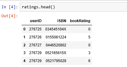
ratings.columns = ['userID', 'ISBN', 'bookRating']

評分資料

評分資料集提供了讀者對於書籍的評分時候資料，有1149780條記錄和3個欄位：userID，ISBN，bookRating。

print(ratings.shape)
print(list(ratings.columns))
(1149780, 3)
['userID', 'ISBN', 'bookRating']

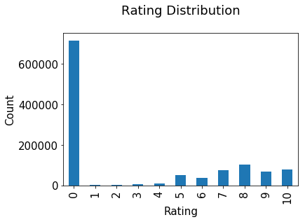
評分分佈

評分分佈非常不均衡，絕大部分都是0。

plt.rc("font", size=15)
ratings.bookRating.value_counts(sort=False).plot(kind='bar')
plt.title('Rating Distribution\n')
plt.xlabel('Rating')
plt.ylabel('Count')
plt.savefig('system1.png', bbox_inches='tight')
plt.show()

圖書資料

圖書資料集提供了很多細節，它包含了271360條記錄，有 ISBN, book title, book author, publisher 等8個欄位。

print(books.shape)
print(list(books.columns))
(271360, 8)
['ISBN', 'bookTitle', 'bookAuthor', 'yearOfPublication', 'publisher', 'imageUrlS', 'imageUrlM', 'imageUrlL']

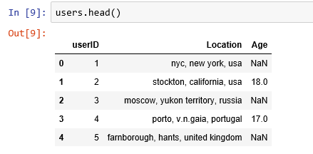
讀者資料

這個資料集提供了讀者的地域資訊，有 user id, location, 和 age 3個欄位，共278858條記錄。

print(users.shape)
print(list(users.columns))
(278858, 3)
['userID', 'Location', 'Age']

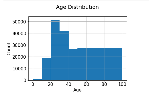
年齡分佈

最活躍的使用者大多20-30歲。

users.Age.hist(bins=[0, 10, 20, 30, 40, 50, 100])
plt.title('Age Distribution\n')
plt.xlabel('Age')
plt.ylabel('Count')
plt.savefig('system2.png', bbox_inches='tight')
plt.show()

基於評分計數的推薦

rating_count = pd.DataFrame(ratings.groupby('ISBN')['bookRating'].count())
rating_count.sort_values('bookRating', ascending=False).head()

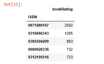
ISBN 號為0971880107的書籍收到了最多的評分，讓我們看看這是本什麼書，再探索下排名前5的書長什麼樣。

most_rated_books = pd.DataFrame(['0971880107', '0316666343', '0385504209', '0060928336', '0312195516'], index=np.arange(5), columns = ['ISBN'])
most_rated_books_summary = pd.merge(most_rated_books, books, on='ISBN')
most_rated_books_summary

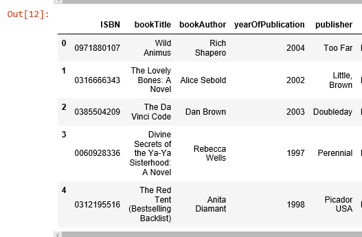
被評分次數最多的書是 Rich Shapero 的 “Wild Animus”，並且排名前5的圖書都是小說。表明小說更受歡迎，並且容易收到評分。如果有人喜歡“The Lovely Bones: A Novel”, 那麼我們應該向他/她推薦 “Wild Animus”。

基於相關性的推薦

我們使用皮爾森相關係數來衡量兩個變數間的線性相關程度，本例中就研究兩本圖書評分的相關性。

首先，我們要計算平均評分和每本書收到的評分個數。

average_rating = pd.DataFrame(ratings.groupby('ISBN')['bookRating'].mean())
average_rating['ratingCount'] = pd.DataFrame(ratings.groupby('ISBN')['bookRating'].count())
average_rating.sort_values('ratingCount', ascending=False).head()

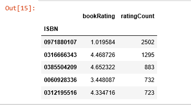
觀測值：在這個圖書資料集裡，收到最多評分的書完全不是評分最高的那些。如果我們只以評分計數為推薦的條件，那麼就錯大發了。因此，我們需要一個更科學的系統。

為保證統計顯著性，收到評分數少於100的圖書和評分次數少於200次的讀者都被排除在外。

counts1 = ratings['userID'].value_counts()
ratings = ratings[ratings['userID'].isin(counts1[counts1 >= 200].index)]
counts = ratings['bookRating'].value_counts()
ratings = ratings[ratings['bookRating'].isin(counts[counts >= 100].index)]

評分矩陣

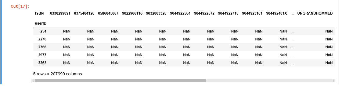
我們將評分轉換為2維矩陣，這個矩陣會很稀疏因為不是每個讀者都對每本書做了評分。

ratings_pivot = ratings.pivot(index='userID', columns='ISBN').bookRating
userID = ratings_pivot.index
ISBN = ratings_pivot.columns
print(ratings_pivot.shape)
ratings_pivot.head()
(905, 207699)

讓我們來尋找被評分次數排名前2的書的相關性。

根據 維基百科，排名第二的書“The Lovely Bones: A Novel”是一個關於一位十幾歲的小姑娘遭遇姦殺，在天堂觀察家人艱辛生活的故事。

bones_ratings = ratings_pivot['0316666343']
similar_to_bones = ratings_pivot.corrwith(bones_ratings)
corr_bones = pd.DataFrame(similar_to_bones, columns=['pearsonR'])
corr_bones.dropna(inplace=True)
corr_summary = corr_bones.join(average_rating['ratingCount'])
corr_summary[corr_summary['ratingCount']>=300].sort_values('pearsonR', ascending=False).head(10)

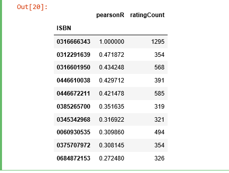
我們獲取了所有書的 ISBN 號，現在我們需要檢視它們的題目是否有資訊。

books_corr_to_bones = pd.DataFrame(['0312291639', '0316601950', '0446610038', '0446672211', '0385265700', '0345342968', '0060930535', '0375707972', '0684872153'], 
                                  index=np.arange(9), columns=['ISBN'])
corr_books = pd.merge(books_corr_to_bones, books, on='ISBN')
corr_books

我們從高度相關的書籍列表中選取3本書，“The Nanny Diaries: A Novel”, “The Pilot’s Wife: A Novel” 和 “Where the Heart is”。 “The Nanny Diaries” 從保姆的視角諷刺了曼哈頓的上層社會。

“The Pilot’s Wife”和“The Lovely Bones”的作者是同一個人，作為非正式三部曲的最後一部，這個故事被設定在新罕布什爾州海岸的一個曾經是修道院的大型海濱別墅中。

“Where the Heart Is” 詳細描述了美國低收入和寄養兒童的苦難。

這三本書聽起來和“The Lovely Bones”有很高的相關性，看起來基於相關性的推薦系統起作用了。

使用基於 KNN 的協同濾波

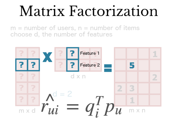
KNN是一個用來基於共同圖書評分以發現相似讀者間聚類狀況的機器學習演算法，並且可以基於距離最近的 k 個鄰居的平均評分來進行預測。舉個例子，我們先看看評分矩陣，該矩陣每一行是一本書每一列是一個讀者：

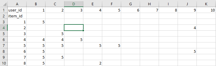
之後我們可以找到讀者行為向量最為相似的k本圖書，本例中 id = 5 的圖書的最近鄰的 id 為 [7, 4, 8, ...]，現在讓我們把這個方法用到推薦系統上。

這次我們只關注那些最為流行的圖書，需要先對圖書在評分這一維度上做些統計工作。

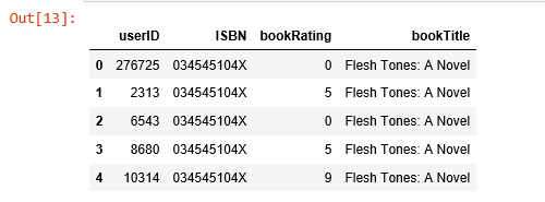
combine_book_rating = pd.merge(ratings, books, on='ISBN')
columns = ['yearOfPublication', 'publisher', 'bookAuthor', 'imageUrlS', 'imageUrlM', 'imageUrlL']
combine_book_rating = combine_book_rating.drop(columns, axis=1)
combine_book_rating.head()

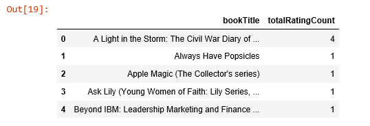
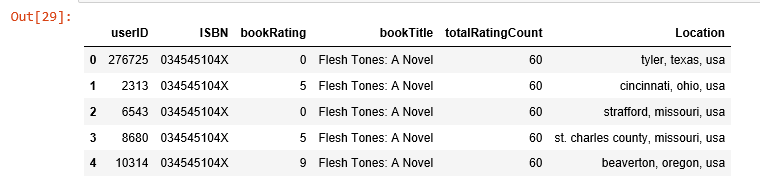
之後我們按照圖書標題分組，並新增一列儲存總的被評分次數。

combine_book_rating = combine_book_rating.dropna(axis = 0, subset = ['bookTitle'])

book_ratingCount = (combine_book_rating.
     groupby(by = ['bookTitle'])['bookRating'].
     count().
     reset_index().
     rename(columns = {'bookRating': 'totalRatingCount'})
     [['bookTitle', 'totalRatingCount']]
    )
book_ratingCount.head()

之後就可以篩選出最流行的書，把那些流傳度不廣的過濾掉。

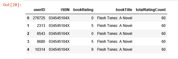
rating_with_totalRatingCount = combine_book_rating.merge(book_ratingCount, left_on = 'bookTitle', right_on = 'bookTitle', how = 'left')
rating_with_totalRatingCount.head()

讓我們看看這些統計量：

pd.set_option('display.float_format', lambda x: '%.3f' % x)
print(book_ratingCount['totalRatingCount'].describe())

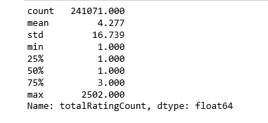
處在中位數位置的數就只被評分一次，讓我們再看看頭部的分佈：

print(book_ratingCount['totalRatingCount'].quantile(np.arange(.9, 1, .01)))

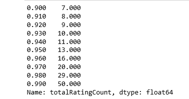
約有1%的書收到了超過50次的評分，由於資料集內記錄眾多，我們就擷取頭部1%的圖書來建模，得到大概2713本書。

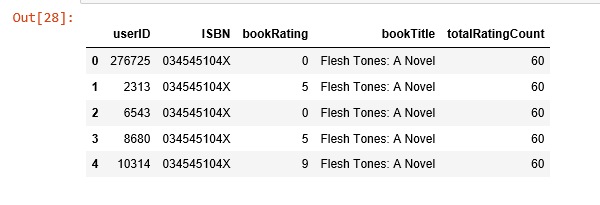
popularity_threshold = 50
rating_popular_book = rating_with_totalRatingCount.query('totalRatingCount >= @popularity_threshold')
rating_popular_book.head()

只保留美國和加拿大的讀者

為了加快計算速度並節約記憶體，我只選取讀者資料集中位於美國和加拿大的資料，然後把這個子集和之前得到的評分資料集合並。

combined = rating_popular_book.merge(users, left_on = 'userID', right_on = 'userID', how = 'left')

us_canada_user_rating = combined[combined['Location'].str.contains("usa|canada")]
us_canada_user_rating=us_canada_user_rating.drop('Age', axis=1)
us_canada_user_rating.head()

應用kNN

我們把資料錶轉化為一個二維矩陣，並把缺失值用0填充（因為要計算評分向量間的距離）。之後我們把矩陣中的評分資料轉化偽scipy庫中的稀疏矩陣來提升計算效率。

尋找近鄰

我們使用sklean.neighbors這一無監督演算法來尋找近鄰，設定“metric=cosine”使得該演算法基於餘弦值來衡量相似度，最後我們再擬合模型。

us_canada_user_rating_pivot = us_canada_user_rating.pivot(index = 'bookTitle', columns = 'userID', values = 'bookRating').fillna(0)
us_canada_user_rating_matrix = csr_matrix(us_canada_user_rating_pivot.values)

from sklearn.neighbors import NearestNeighbors

model_knn = NearestNeighbors(metric = 'cosine', algorithm = 'brute')
model_knn.fit(us_canada_user_rating_matrix)
NearestNeighbors(algorithm='brute', leaf_size=30, metric='cosine',
         metric_params=None, n_jobs=1, n_neighbors=5, p=2, radius=1.0)

測試模型並做些推薦

這一步驟，kNN演算法會計算距離作為例項間的近似度，然後找到例項的近鄰，用近鄰類別中的多數類對其進行分類。

query_index = np.random.choice(us_canada_user_rating_pivot.shape[0])
distances, indices = model_knn.kneighbors(us_canada_user_rating_pivot.iloc[query_index, :].reshape(1, -1), n_neighbors = 6)

for i in range(0, len(distances.flatten())):
    if i == 0:
        print('Recommendations for {0}:\n'.format(us_canada_user_rating_pivot.index[query_index]))
    else:
        print('{0}: {1}, with distance of {2}:'.format(i, us_canada_user_rating_pivot.index[indices.flatten()[i]], distances.flatten()[i]))
Recommendations for the Green Mile: Coffey's Hands (Green Mile Series):

1: The Green Mile: Night Journey (Green Mile Series), with distance of 0.26063737394209996:
2: The Green Mile: The Mouse on the Mile (Green Mile Series), with distance of 0.2911623754404248:
3: The Green Mile: The Bad Death of Eduard Delacroix (Green Mile Series), with distance of 0.2959542871302775:
4: The Two Dead Girls (Green Mile Series), with distance of 0.30596709534565514:
5: The Green Mile: Coffey on the Mile (Green Mile Series), with distance of 0.37646848777592923:

完美！Green Mile 系列圖書就該逐一被推薦。

使用矩陣分解進行協同濾波

矩陣分解是一種常用的數學工具，這一技術非常有用，因為它使得使用者可以發現讀者和使用者間的潛在互動特徵。

本例我們將使用SVD分解，這是一種發現潛在因子的常用方法。

與kNN類似，我們把美國和加拿大讀者的評分錶轉換為二維矩陣（命名為效用矩陣）並把缺失值用0填充。

us_canada_user_rating_pivot2 = us_canada_user_rating.pivot(index = 'userID', columns = 'bookTitle', values = 'bookRating').fillna(0)
us_canada_user_rating_pivot2.head()

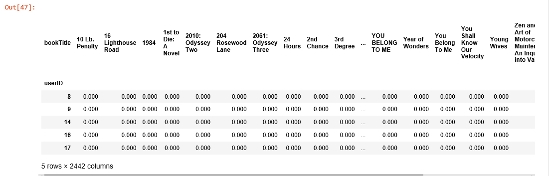
之後我們將效用矩陣轉置，每行是圖書標題，每列是讀者ID。用 TruncatedSVD 對其進行分解之後，我們出於降維的目的擬合模型。由於我們要保留圖書標題，現在這一過程是針對矩陣的列進行的。我們設定 n_components = 12 來尋找12個潛在變數，這樣我們的維度就從40017 X 2442 降至 2442 X 12。

us_canada_user_rating_pivot2.shape
(40017, 2442)

X = us_canada_user_rating_pivot2.values.T
X.shape
(2442, 40017)

import sklearn
from sklearn.decomposition import TruncatedSVD

SVD = TruncatedSVD(n_components=12, random_state=17)
matrix = SVD.fit_transform(X)
matrix.shape
(2442, 12)

在最終的矩陣中，我們計算了每兩本書之間的皮爾森相關係數，為了比較它與kNN的效果，我們以 “The Green Mile: Coffey’s Hands (Green Mile Series)”作為案例，尋找和他相關係數（0.9到1之間）最高的書。

import warnings
warnings.filterwarnings("ignore",category =RuntimeWarning)
corr = np.corrcoef(matrix)
corr.shape
(2442, 2442)

us_canada_book_title = us_canada_user_rating_pivot2.columns
us_canada_book_list = list(us_canada_book_title)
coffey_hands = us_canada_book_list.index("The Green Mile: Coffey's Hands (Green Mile Series)")
print(coffey_hands)
1906

看到了吧！

corr_coffey_hands  = corr[coffey_hands]
list(us_canada_book_title[(corr_coffey_hands0.9)])
['Needful Things',
 'The Bachman Books: Rage, the Long Walk, Roadwork, the Running Man',s
 'The Green Mile: Coffey on the Mile (Green Mile Series)',
 'The Green Mile: Night Journey (Green Mile Series)',
 'The Green Mile: The Bad Death of Eduard Delacroix (Green Mile Series)',
 'The Green Mile: The Mouse on the Mile (Green Mile Series)',
 'The Shining',
 'The Two Dead Girls (Green Mile Series)']

不謙虛地說，這個系統可以打敗亞馬遜的推薦系統，你覺得呢?

參考文獻：

Music RecommendationsohAI

原文連結