感知機是1957年由Rosenblatt提出，是神經網路與支援向量機的基礎，是二類分類的線性分類模型。

感知器模型

     適用問題：二類分類

     模型特點：分離超平面

     模型型別：判別模型

感知機學習策略

     學習策略：極小化誤分點到超平面距離   

     學習的損失函式：誤分點超平面距離

感知機學習演算法

     學習演算法：隨機梯度下降

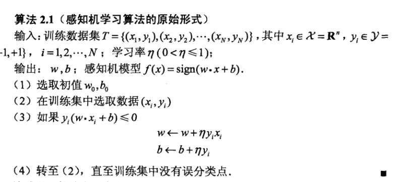
演算法中感知器模型是一個sigmoid函式，於是上述模型是一個二分類的線性分類器。

資料集介紹

我們選擇MNIST資料集進行實驗

MNIST是一個入門級的計算機視覺資料集，它包含各種手寫數字圖片：

它也包含每一張圖片對應的標籤，告訴我們這個是數字幾。比如，上面這四張圖片的標籤分別是5，0，4，1。

其官方下載地址：http://yann.lecun.com/exdb/mnist/

但是原始資料太麻煩了，我們選擇kaggle提供的已處理好的資料
地址：https://www.kaggle.com/c/digit-recognizer/data

由於我們是二分類器，所以需要對train.csv中的label列進行一些微調，label等於0的繼續等於0，label大於0改為1。

這樣就將十分類的資料改為二分類的資料。
也可以從我的github上下載：https://github.com/WenDesi/lihang_book_algorithm/blob/master/data/train_binary.csv

HOG特徵提取

MNIST資料都是28*28的圖片，可選擇的特徵有很多，包括：
1. 自己提取特徵
2. 將整個圖片作為特徵向量
3. HOG特徵

我們選擇HOG特徵，HOG特徵相關內容大家可以參考zouxy09 的相關博文

我們的目標是實用！因此只展示如何用Python提取HOG特徵。

Python提取特徵需要呼叫opencv2，程式碼如下所示

hog = cv2.HOGDescriptor('../hog.xml')
img = np.reshape(img,(28,28))
cv_img = img.astype(np.uint8)
hog_feature = hog.compute(cv_img)

其中hog.xml儲存hog的配置資訊，如下所示

<?xml version="1.0"?>
<opencv_storage>
<hog type_id="opencv-object-detector-hog">
  <winSize>
    28 28</winSize>
  <blockSize>
    14 14</blockSize>
  <blockStride>
    7 7</blockStride>
  <cellSize>
    7 7</cellSize>
  <nbins>9</nbins>
  <derivAperture>1</derivAperture>
  <winSigma>4.</winSigma>
  <histogramNormType>0</histogramNormType>
  <L2HysThreshold>2.0000000000000001e-001</L2HysThreshold>
  <gammaCorrection>1</gammaCorrection>
  <nlevels>64</nlevels></hog>
</opencv_storage>

關於更多hog特徵配置資訊，大家可以參考這篇文章

程式碼

程式碼我已經放到Github上了，大家可以參考我的Github:https://github.com/WenDesi/lihang_book_algorithm

感知器程式碼位於perceptron/binary_perceptron.py

這裡也貼一下程式碼

#encoding=utf-8

import pandas as pd
import numpy as np
import cv2
import random
import time

from sklearn.cross_validation import train_test_split
from sklearn.metrics import accuracy_score

# 利用opencv獲取影象hog特徵
def get_hog_features(trainset):
    features = []

    hog = cv2.HOGDescriptor('../hog.xml')

    for img in trainset:
        img = np.reshape(img,(28,28))
        cv_img = img.astype(np.uint8)

        hog_feature = hog.compute(cv_img)
        # hog_feature = np.transpose(hog_feature)
        features.append(hog_feature)

    features = np.array(features)
    features = np.reshape(features,(-1,324))

    return features

def Train(trainset,train_labels):
    # 獲取引數
    trainset_size = len(train_labels)

    # 初始化 w,b
    w = np.zeros((feature_length,1))
    b = 0

    study_count = 0                         # 學習次數記錄，只有當分類錯誤時才會增加
    nochange_count = 0                      # 統計連續分類正確數，當分類錯誤時歸為0
    nochange_upper_limit = 100000           # 連續分類正確上界，當連續分類超過上界時，認為已訓練好，退出訓練

    while True:
        nochange_count += 1
        if nochange_count > nochange_upper_limit:
            break

        # 隨機選的資料
        index = random.randint(0,trainset_size-1)
        img = trainset[index]
        label = train_labels[index]

        # 計算yi(w*xi+b)
        yi = int(label != object_num) * 2 - 1                       # 如果等於object_num, yi= 1, 否則yi=1
        result = yi * (np.dot(img,w) + b)

        # 如果yi(w*xi+b) <= 0 則更新 w 與 b 的值
        if result <= 0:
            img = np.reshape(trainset[index],(feature_length,1))    # 為了維數統一，需重新設定一下維度

            w += img*yi*study_step                                  # 按演算法步驟3更新引數
            b += yi*study_step

            study_count += 1
            if study_count > study_total:
                break
            nochange_count = 0
    return w,b

def Predict(testset,w,b ):
    predict = []
    for img in testset:
        result = np.dot(img,w) + b
        result = result > 0
        predict.append(result)
    return np.array(predict)

study_step = 0.0001                                 # 學習步長
study_total = 10000                                 # 學習次數
feature_length = 324                                # hog特徵維度
object_num = 0                                      # 分類的數字

if __name__ == '__main__':

    print 'Start read data'

    time_1 = time.time()

    raw_data = pd.read_csv('../data/train_binary.csv',header=0)
    data = raw_data.values

    imgs = data[0::,1::]
    labels = data[::,0]

    features = get_hog_features(imgs)

    # 選取 2/3 資料作為訓練集， 1/3 資料作為測試集
    train_features, test_features, train_labels, test_labels = train_test_split(features, labels, test_size=0.33, random_state=23323)
    # print train_features.shape
    # print train_features.shape

    time_2 = time.time()
    print 'read data cost ',time_2 - time_1,' second','\n'

    print 'Start training'
    w,b = Train(train_features,train_labels)
    time_3 = time.time()
    print 'training cost ',time_3 - time_2,' second','\n'

    print 'Start predicting'
    test_predict = Predict(test_features,w,b)
    time_4 = time.time()
    print 'predicting cost ',time_4 - time_3,' second','\n'

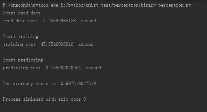
    score = accuracy_score(test_labels,test_predict)
    print "The accruacy socre is ", score

執行結果如下所示，可以看到準確度還不錯

演算法的收斂性

      證明：Novikoff定理

演算法的對偶形式

      為了求解更簡單，所以用對偶形式