影象處理的變分法研究（1）——11月第一階段進展報告

按：10.30——11.8（共10天）階段性報告（開題答辯後一個星期）這部分的筆記看紙質的比較好，總結的較好些。

一、總變分的物理數學背景

參考資料：（1）Gilboa的課程Variational Methods in Image Processing. Course Website 主要是notes1—notes5, exercise1 & exercise2(TVBD部分)
(2)馮象初《影象處理的變分和偏微分方程》chap1 & chap2
(3)Gilboa推薦的數學書籍《Mathematical Problems in Image Processing:Partial Differential Equations and the Calculus of Variations》影象處理中的數學問題chap2 & chap3
(4)PPT 《數學物理方程》學生群裡下載的國科大的，關於變分法那一章。另外配套的教材裡也有變分法一章，有一些基本推導，可以加強理解。

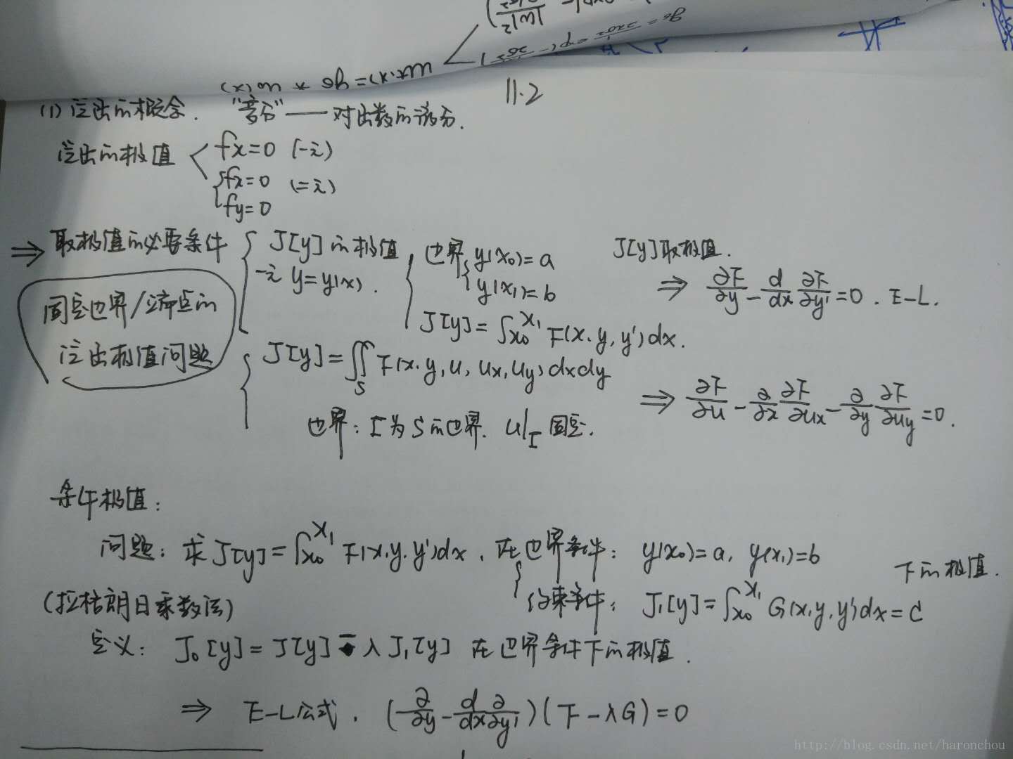
泛函的概念、泛函極值

變分——就是泛函J對函式u的微分。泛函——自變數是函式，因變數是一個值，達到一一對應。泛函極值——求一個最佳的函式使得因變數取最大值。因此，對J(u)泛函求極值，要對J(u)求微分（二元時求偏導），就是變分了。
——可以推導，無論一元還是二元，minJ(u)當滿足E-L公式時，取得極值。得到E-L公式後，就是求解這個公式，方法是用時間演化，即ut = E-L = 0. 其中dt的取值有限制，要滿足CFL條件。

物理學上的泛函

三類典型的數學物理方程都是偏微分方程。邊界條件+初始條件才能確定解。

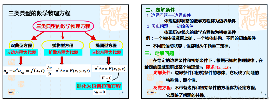
​ 其中，我們的擴散方程與我們影象處理息息相關。
在馮象初《書》中，我們可以總結：div(c gradu)=0是線性擴散，係數為常數。c = 1時的擴散方程，ut = gradu。這個方程的解 == 用高斯函式與U卷積表示。其中高斯函式:σ=2t−−√

。這一證明可見matlab程式碼：haron_LinearDiffusion.m 確實線性擴散收斂後的結果與高斯卷積模糊的結果是一樣的。（程式碼1，貼圖）。

ut=Δu=uxx+uyy

u_t = \Delta{u} = u_{xx}+u_{yy}

線性擴散: div(c×u(x))

div(c\times u(x))

，其中c=1

c =1

, un+1=un+dt×(Δu)

u^{n+1} = u^n+dt\times(\Delta u)

.
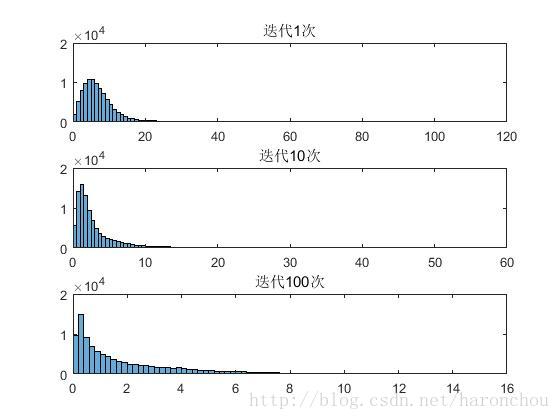
其中，根據迭代過程的收斂性看，100次已經達到了穩定。

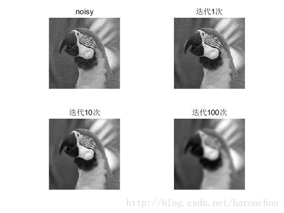
由於線性擴散與高斯卷積等價，可以看出經歷相同時間t後，線性擴散收斂後的結果與高斯平滑的結果一致，它們的差如第四張圖。

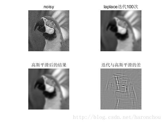
這個是線性擴散迭代後的估計影象的直方圖分佈，可以看出隨著迭代的進行，直方圖越來越平坦，意味著影象被平滑掉了。

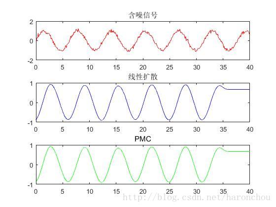
一維訊號用線性擴散和PMC去噪的結果，兩者類似（其中高斯噪聲標準差為10）。注意：這裡dt時間步長的選擇對迭代次數有關，PMC中K值的選擇跟噪聲標準差有關。目前只能手動選擇看效果，如何設計演算法自動選擇最佳的引數值有待研究。

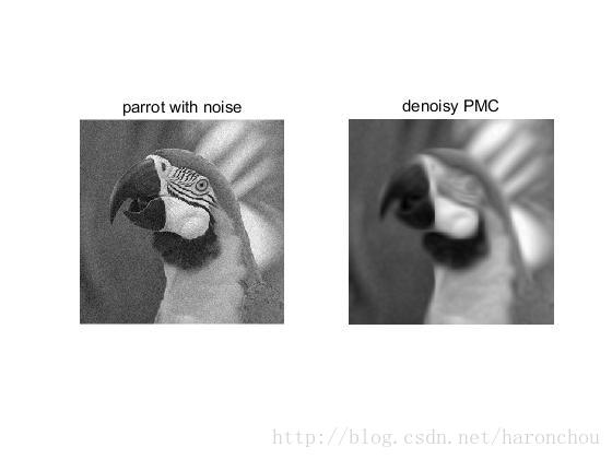
這裡是PMC用在二維影象上的效果。

​ 那麼，下面我們要做的是：根據方法的不同，我們設計了不同的泛函（能量泛函），求出相應的E-L公式。最後我們需要求解E-L方程。人們還設計了不同的求解方法去求解E-L。也有不同的方法去離散E-L方程，如：有限元法、有限差分、？（忘了）等。

​ 下一步工作計劃：找出有哪些不同的泛函（對應的物理解釋）、相應的E-L方程、如何求解E-L？最後Matlab實現這些方法、採用一定的評價指標評價這些方法、總結優缺點、找到自己的突破點！

​ 這些計劃的資訊來源：歷年博碩士論文（優秀的）——為了得到關於其基本理論的闡述：如變分法的發展（哪些人做了哪些修改、效果、基本原理、他們的英文文章來源等）。

自我總結與評價

​ 這段時間的工作非常基礎，但是似乎與主要工作方向偏離了。看了很多資料（英文），看了很多理論，寫了很多筆記，寫了一點點程式碼(這部分基礎程式碼還是對理解有幫助的！)。還沒有得到我最想要的東西，最想看的最想總結的，接下來的半個月要加油！

程式碼1 比較線性擴散和高斯卷積

%%
%要求1：作為時間的函式，計算和繪製下列度量的圖
%               （1）標準偏差
%               （2）時間t在0.1,1,10時， 影象的梯度幅度值的三個直方圖。
%       解釋其趨勢及發生原因
%要求2：將擴散與等效sigma的高斯卷積相比較。如有差異解釋原因
%%結論： 擴散與高斯卷積的結果大致相同，略微差別。
%%
f_parrot = imread('parrot.png');
f_parrot = double(rgb2gray(f_parrot));
% imshow(f_girl,[0,255]), title('Original girl image');
%加噪聲
N_std = 10; % noise standard deviation
noise = randn(size(f_parrot))*N_std;
f = f_parrot + noise;
% figure(2); imshow(f,[0,255]), title('Sun-girl with noise');
C = 1;
%%
%畫t=0.1,1,10處的梯度值的直方圖
dt = 0.1;
Iter1 =1;
u1 = diffusion_lin(f,C, Iter1, dt);
grad1 = gradF(u1);
u2 = diffusion_lin(f,C, Iter1*10, dt);
grad2 = gradF(u2);
[u3, J3] = diffusion_lin(f,C, Iter1*100, dt);
grad3 = gradF(u3);
%畫圖顯示
figure(1);
t = 0:0.01:10;
plot(t, sqrt(2*C*t),'r');legend('sqrt(2*C*t)');xlabel('t'), ylabel('\sigma(t)');
figure(2);
subplot(221);imshow(f,[]),title('noisy');
subplot(222);imshow(u1,[]),title('迭代1次');
subplot(223);imshow(u2,[]),title('迭代10次');
subplot(224);imshow(u3,[]),title('迭代100次');
figure(3);
subplot(311); histogram(grad1);title('迭代1次');
subplot(312);histogram(grad2);title('迭代10次');
subplot(313); histogram(grad3);title('迭代100次');
%%
figure(4);
plot(1:100, J3, 'b');
%%
%%高斯核卷積對比
n = 100;
t = n * dt;
gauss = fspecial('gaussian',size(f),sqrt(2*t));
u_gaussian = imfilter(f, gauss, 'symmetric');
figure(5);
imshow(u_gaussian,[]), title('高斯平滑後的結果');
u_difference = u3 - u_gaussian;
figure(6); imshow(u_difference,[]),
title('迭代與高斯平滑的差');
%%
function grad_f = gradF(f)
[nx ny] = size(f);
f_x = (f(:,[2:nx nx])-f(:,[1 1:nx-1]))/2;
f_y = (f([2:ny ny],:)-f([1 1:ny-1],:))/2; 
grad_f = (sqrt(f_x.^2+f_y.^2));
end

%%
function [u, J]=diffusion_lin(f,C,Iter,dt)
% u=diffusion_lin(f,C,Iter,dt)  線性擴散 Sun-girl 影象
% parameters:
% f      = input image (2D gray-level)
% C      = constant diffusion coefficient
% Iter   = number of iterations 
% dt     = time step 
I = f;%讀入影象
[nx ny] = size(f);
for i = 1: Iter
     Iold = I;
     I_xx = I(:,[2:nx nx])+I(:,[1 1:nx-1])-2*I;%二階微分
     I_yy = I([2:ny ny],:)+I([1 1:ny-1],:)-2*I;
     I_t = C * (I_xx + I_yy);
     I = I + dt* I_t;
     Inew = I;
     J(i) = norm(Iold - Inew);
end
u = I;
end

%%part1：一維降噪，線性和PMC
t = 0:0.1:40;
y_true = sin(t);
%加噪聲
N_std = 0.1; % noise standard deviation
noise = randn(size(y_true))*N_std;
y = y_true + noise;
subplot(311);plot(t,y,'r');title('含噪訊號')
%%線性擴散
dt = 0.5;%[0,1]之間
Iter = 100;
[u1, J1] = diffusion_lin1D(y, 1, Iter, dt);
subplot(312);plot(t,u1,'b');title('線性擴散');
K = 2;
[u2, J2] = diffusion_PMC(y, K, Iter, dt);
subplot(313);plot(t,u2,'g');title('PMC');
figure;plot(1:Iter, J1,'b');hold on;plot(1:Iter, J2,'r');legend('Linear','PMC')
function [u, J] = diffusion_PMC(f,K,Iter,dt)
%公式推導見Exercise1
[nx ny] = size(f);
for i = 1: Iter
    fold = f;
    f_xx = f([2:ny ny])+f([1:ny-1 ny-1]) -2*f;
    f_x = (f([2:ny ny]) - f([1:ny-1 ny-1])) / 2;
    temp = ((f_x ./ K).^2 + 1 ) .^1.5;
    f_t = f_xx ./ temp;
    fnew = fold + dt.* f_t;
    f = fnew;
    J(i) =norm(fold - fnew);
end
   u = f;
end

function [u, J]=diffusion_lin1D(f,C,Iter,dt)
% u=diffusion_lin(f,C,Iter,dt)  線性擴散 Sun-girl 影象
% parameters:
% f      = input image (2D gray-level)
% C      = constant diffusion coefficient
% Iter   = number of iterations 
% dt     = time step 
I = f;%讀入影象
[nx ny] = size(f);
for i = 1: Iter
     Iold = I;
     I_xx = I([2:ny ny])+I([1:ny-1 ny-1]) -2*I;%二階微分
     I_t = C * (I_xx);
     I = I + dt* I_t;
     Inew = I;
     J(i) = norm(Iold - Inew);
end
u = I;
end

close all, clc;
f_parrot = imread('parrot.png');
f_parrot = double(rgb2gray(f_parrot));
% imshow(f_girl,[0,255]), title('Original girl image');
%加噪聲
N_std = 10; % noise standard deviation
noise = randn(size(f_parrot))*N_std;
f = f_parrot + noise;
% figure(2); imshow(f,[0,255]), title('parrot with noise');
K =10;
Iter = 100;
dt = 0.01;
[u1, J1] = diffusion_PMC(f, K, Iter, dt);
subplot(121),imshow(f,[]),title('parrot with noise');
subplot(122),imshow(u1,[]),title('denoisy PMC');
figure;plot(1:Iter, J1);
%PMC降噪
function [u, J] = diffusion_PMC(f,K,Iter,dt)
%公式推導見Exercise1
[nx ny] = size(f);
for i = 1: Iter
    fold = f;
     f_x = (f(:,[2:nx nx])-f(:,[1 1:nx-1]))/2;
    f_y = (f([2:ny ny],:)-f([1 1:ny-1],:))/2;
    f_xx = f(:,[2:nx nx])+f(:,[1 1:nx-1])-2*f;
    f_yy = f([2:ny ny],:)+f([1 1:ny-1],:)-2*f;
    A = (1 + (f_x.^2 + f_y.^2)./ K.^2) .^1.5;
    temp = (1 + f_x .^2) .* f_yy + (1 + f_y .^2) .* f_xx;
    f_t = temp ./ A;
    fnew = fold + dt.* f_t;
    f = fnew;
    J(i) =norm(fold - fnew);
end
   u = f;
end