八大排序簡單小結及c++實現

   即插入排序、氣泡排序、選擇排序、shell排序、基數排序、歸併排序、快速排序、堆排序

一、（直接）插入法(交換排序) 

1、原理方法

       從第二個數開始與前面的一個一個比較，小於則交換、大於等於則下一個數的迴圈。

2、特點

1）、穩定性：穩定

2）、時間代價：O(n*n)

    最好——正序——時間代價Θ(n)    

    最差——倒序——時間代價Θ(n*n)  

    平均——亂序——時間代價Θ(n*n) 

3）、輔助儲存空間：O(1)

4）、比較

①較為複雜、速度較慢

②n較小時(如<=50) 、區域性或整體有序時適用

   插入排序的最佳時間代價特性——基本有序。

③迴圈交換

迴圈不同：f(n)<=1/2*n*(n-1)<=1/2*n*n

交換不同(賦值操作)

3、程式碼

#include <iostream>
using namespace std;

void InsertSort(int*  , int );
int main() 
{ 	
    int data[]={1,-30,12,7,-1,5,4};
    InsertSort(data,7);
    for(int i=0;i<7;i++)
        cout<<dec<<data[i]<<"  ";
        cout<<"\n";
    //system ( "pause" );//getchar();
    return 0;
 } 

void  InsertSort(int* pData,int Count)
{
    int iTemp;
　　int iPos;
    for(int i=1;i<Count;i++)
    {
        iPos=i-1;
        iTemp=pData[i];
        while((iPos>=0)&&(iTemp<pData[iPos]))
        {
            pData[iPos+1]=pData[iPos];
            iPos--;
        }
        pData[iPos+1]=iTemp; 
    }
}

二、冒泡法(交換排序)

1、原理方法

1）、把小的元素往前調或者把大的元素往後調， 一趟得到一個最大值或最小值。

          若迴圈外設一個bool變數、最差(倒序)迴圈n-1趟、最好(正序)迴圈一趟

2）、有遞迴和非遞迴實現

2、特點

1）、穩定性：穩定

2）、時間代價：

    最好——正序、無交換（O(0)）——時間代價Θ(n)（只迴圈一趟）

    最差——倒序、迴圈次數=交換次數（O(n*n)）——時間代價Θ(n*n)  

    平均——亂序、中間狀態                  ——時間代價Θ(n*n)  

3）、輔助儲存空間：O(1)

4）、比較

①速度較慢、交換次數相對比較多

②n較小時(如<=50) ，區域性或整體有序時、較快

③迴圈交換

迴圈相同(若迴圈外不設判斷條件)：

           1+2+...+n-1=1/2*(n-1)*n<=1/2*n*n＝K*g(n)

              f(n)＝O(g(n))＝O(n*n)(迴圈複雜度)

交換不同

3、程式碼

1）、非遞迴迴圈實現

#include <iostream>
using namespace std;

void BubbleSort(int*  , int );
int main() 
{ 	
    int data[]={10,9,13,7,32,5,2};
    BubbleSort(data,7);
    for(int i=0;i<7;i++)
        cout<<dec<<data[i]<<"  ";
        cout<<"\n";
    return 0;
 } 

void  BubbleSort(int* pData,int n)
{
　　int iTemp;

    bool bFilish=fale;
    for(int i=0;i<n-1;i++)
　　{
        if(bFlish=true)
            break;
        bFilish=true;
        for(int j=n-1;j>i;j--)
        {
            if(pData[j]<pData[j-1])
            {
                iTemp=pData[j-1];
                pData[j-1]=pData[j];
                pData[j]=iTemp;
                bFilish=false;
            }

        }
    }
}

2）、遞迴，下面採用雙向冒泡

#include <iostream>
using namespace std;

void BilateralBubbleSort(int*  , int,int );
int main() 
{ 	
    int data[]={10,9,13,7,32,5,2};
    BilateralBubbleSort(data,0,6);
    for(int i=0;i<7;i++)
        cout<<dec<<data[i]<<"  ";
        cout<<"\n";
    return 0;
} 

void BilateralBubbleSort(int *a, int first, int last) 
{
    if (first >= last) //退出條件
    {                          
         return;
    }

    int i = first;
    int j = last;
    
    int temp = a[first];    
    while (i != j) 
    {                            
        while (i<j && a[j]>=temp)  
        {
            j--;
        }
        a[i] = a[j];
        while (i<j && a[i]<=temp) 
        {
            i++;
        }
        a[j] = a[i];
    }
    a[i] = temp;

    //遞迴，有點像快速排序，就是中間值放在臨時變數而不是陣列尾部
    BilateralBubbleSort(a, first, i-1);     
    BilateralBubbleSort(a, i+1, last);
  
}

三、（簡單或直接）選擇法(交換排序)

1、原理方法

1）、第一個元素開始，同其後的元素比較並記錄最小值(放在當前位置)。

         每次得到一個最小值

2）、(改進)選擇中間變數、減少交換次數

2、特點

1）、穩定性：不穩定

2）、時間代價：O(n*n)

    最好——正序、無交換（O(0)）                

    最差——倒序、迴圈次數=交換次數

    平均—— 亂序、中間狀態                  

3）、輔助儲存空間：O(1)

4）、比較

①速度較慢

②與冒泡法某些情況下稍好，在某些情況下稍差

  這3種中是很有效的， n較小時(如<=50) 適用

③迴圈交換

迴圈相同：

         1/2*(n-1)*n

交換不同

3、程式碼

#include <iostream>
using namespace std;

void SelectSort(int*  , int );
int main() 
{ 	
    int data[]={1,9,12,7,26,5,4};
    SelectSort(data,7);
    for(int i=0;i<7;i++)
	cout<<dec<<data[i]<<"  ";
    cout<<"\n";
    return 0;
} 

void  SelectSort(int* pData,int Count)
{
    int iTemp;
    for(int i=0;i<Count-1;i++)
    {
	for(int j=i+1;j<Count;j++)
	{
	    if(pData[i]<pData[j])
	    {
		iTemp=pData[i];
		pData[i]=pData[j];
		pData[j]=iTemp;
	    }
	}
    }
}

四、快速排序

 1、原理方法

1）、分治法

2）、二叉查詢樹

像一個二叉樹、遞迴實現

①(分割)首先選擇一個軸值，如放在陣列最後

②把比它小的放在左邊，大的放在右邊（兩端移動下標，找到一對後交換）。

③直到相遇、返回下標k(右半部起始、即軸值下標)

④然後對兩邊分別使用這個過程

3）、軸值的選取

①第一個記錄的關鍵碼(正、逆序時有問題)

②隨機抽取軸值(開銷大)

③陣列中間點(一般)

4）、最理想的情況
①陣列的大小是2的冪，這樣分下去始終可以被2整除

    假設為2的k次方，即k＝log2(n)。 

②每次我們選擇的值剛好是中間值、陣列可以被等分。 

第一層遞迴，迴圈n次，第二層迴圈2*(n/2)...... 
所以共有n+2(n/2)+4(n/4)+...+n*(n/n) ＝ n+n+n+...+n＝k*n＝log2(n)*n 
所以演算法複雜度為O(n*log2(n)) 

其他的情況只會比這種情況差，最差的情況是每次選擇到的middle都是最小值或最大值，那麼他將變成交換法（由於使用了遞迴，情況更糟）。

 2、特點

1）、穩定性：不穩定

2）、時間代價：O(n*logn) 

   最差——O(n*n) 

    平均——O(n*logn)，介於最佳和最差之間

    最好——O(n*logn)

3）、輔助儲存空間：O(logn)

4）、比較

 ①區域性或整體有序時慢

 ②(大多數情況)平均最快

   n(≥9)較大時、關鍵字元素比較隨機（雜亂無序）適用

 ③分割陣列，多交換、少比較

3、程式碼

1）、一般的方法

#include<iostream>
using namespace std;
typedef int* IntArrayPtr;

int Divide(int a[],int left,int right)
{
    int k=a[left];  //軸值
    do
    {
	while(left<right&&a[right]>=k) --right;
        if(left<right)
        {
	    a[left]=a[right];
	    ++left;
        }
      
	while(left<right&&a[left]<=k)++left;
	if(left<right)
	{
	    a[right]=a[left];
	    --right;
	}
    }while(left!=right);
    //排序後軸值位置，分為兩個子序列
    a[left]=k;
    return left;
}

void QuickSort(int a[],int left,int right)
{
    int mid;
    if(left>=right)return;

    mid=Divide(a,left,right);
    cout<<a[mid]<<'\n';
    for(int j=left;j<=right;j++)
	cout<<a[j]<<" ";
    cout<<'\n';

        //軸值左半部分
    QuickSort(a,left,mid-1);
        //軸值右半部分
    QuickSort(a,mid+1,right);
}

void FillArray(int a[],int size)//輸入資料
{
    cout<<"請輸入"<<size<<"個整數，數字之間用空格隔開:"<<endl;
    for(int index=0;index<size;index++)
	cin>>a[index];
}

void main()
{
    int array_size;
    cout<<"請輸入需要排序的元素個數：";
    cin>>array_size;
    IntArrayPtr a;
    a=new int[array_size];//動態陣列
	
    FillArray(a,array_size);
    cout<<'\n'<<"快速排序開始："<<endl;
    
    QuickSort(a, 0, array_size-1);
    cout<<"end"<<'\n';
    for(int k=0;k<array_size;k++)
    {
	cout<<a[k]<<" ";
    }
    cout<<'\n';
    system("pause");//getchar();
}

2）、劍指offer上一個比較好的方法，儲存了陣列的兩個位置index向前遍歷陣列，small用於儲存交換的小於軸值的數，找到一個前移一步。

#include "stdafx.h"
#include <stdlib.h>
#include <exception>

int RandomInRange(int min, int max)   //隨機軸值
{
    int random = rand() % (max - min + 1) + min;
    return random;
}

void Swap(int* num1, int* num2)
{
    int temp = *num1;
    *num1 = *num2;
    *num2 = temp;
}

int Partition(int data[], int length, int start, int end)
{
    if(data == NULL || length <= 0 || start < 0 || end >= length)   
        throw new std::exception("Invalid Parameters");

    int index = RandomInRange(start, end);
    Swap(&data[index], &data[end]);

    int small = start - 1;
    for(index = start; index < end; ++ index)   
    {
        if(data[index] < data[end])
        {
            ++ small;
            if(small != index)   
                Swap(&data[index], &data[small]);
        }
    }

    ++ small;     
    Swap(&data[small], &data[end]);

    return small;
}

//遞迴快速排序
void QuickSort(int data[], int length, int start, int end)
{
    if(start=end)
        reurn;

    int index=Partition(data, length, start, end);   
    if(index>start)
        QuickSort(data, length, start, index-1);
    if(index<end)
        QuickSort(data, length,  index+1.end);
}

五、Shell排序（縮小增量排序）(區域性用的插入排序)

1、原理方法

       由於複雜的數學原因避免使用2的冪次步長，它能降低演算法效率

        子序列——每輪等數量（大到小）、等增量、等長度——插入排序——合併再重複

實現：

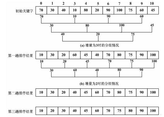
（1）初始增量為3，該陣列分為三組分別進行排序。（初始增量值原則上可以任意設定 

    （0<gap<n），沒有限制）

（2）將增量改為2，該陣列分為2組分別進行排序。

（3）將增量改為1，該陣列整體進行排序。

 

2、特點

1）、穩定性：不穩定

2）、時間代價——依賴於增量序列

                                                   最好                            最差

 

  平均——(約)增量除3時是O（n1.5）、O(n*logn}～O（n2）

3）、輔助儲存空間：O(1)

4）、比較

    ①規模非常大的資料排序不是最優選擇

    ②n為中等規模時是不錯的選擇

 3、程式碼

#include <iostream>
using namespace std;

int a[] = {70,30,40,10,80,20,90,100,75,60,45};
void shell_sort(int a[],int n);

int main()
{
    cout<<"Before Sort: ";
    for(int i=0; i<11; i++)
	cout<<a[i]<<" ";
    cout<<endl;
    shell_sort(a, 11);
    cout<<"After Sort: ";
    for(int i=0; i<11; i++)
	cout<<a[i]<<" ";
    cout<<endl;
    system("pause");  //getchar();//gcc中沒有system("pause");命令
}

void shell_sort(int a[], int n)
{
    for(int gap = 3; gap >0; gap--)
   {
       for(int i=0; i<gap; i++)
       {
	    for(int j = i+gap; j<n; j=j+gap)
	   {
		if(a[j]<a[j-gap])
		{
		    int temp = a[j];
		    int k = j-gap;
		    while(k>=0&&a[k]>temp)
		    {
			a[k+gap] = a[k];
			k = k-gap;
		    }
		    a[k+gap] = temp;
		}
	    }
        }
    }
}

六、歸併排序

 1、原理方法

分治法、歸併操作（演算法）、穩定有效的排序方法(直接插入)、等長子序列

1）、歸併操作。

設有數列{6，202，100，301，38，8，1}

初始狀態：6,202,100,301,38,8，1

第一次歸併後：{6,202},{100,301},{8,38},{1}，比較次數：3；

第二次歸併後：{6,100,202,301}，{1,8,38}，比較次數：4；

第三次歸併後：{1,6,8,38,100,202,301},比較次數：4；

總的比較次數為：3+4+4=11,；

逆序數為14；

2）、將已有序的子序列合併，得到完全有序的序列。若將兩個有序表合併成一個有序表，稱為二路歸併。

3）、非遞迴演算法實現

假設序列共有n個元素。

①將序列每相鄰兩個數字進行歸併操作（merge)，形成floor(n/2)個序列，排序後每個序列包含兩個元素

②將上述序列再次歸併，形成floor(n/4)個序列，每個序列包含四個元素

③重複上面步驟，直到所有元素排序完畢

 2、特點

1）、穩定性：穩定

2）、時間代價：O(n*logn)

3）、輔助儲存空間：O(N)

4）、比較

①空間允許的情況下O(n)

②速度僅次於快速排序、n較大、有序時適用

排序：一般用於對總體無序，但是各子項相對有序的數列

求逆序對數：具體思路是，在歸併的過程中計算每個小區間的逆序對數，進而計算出大區間的逆序對數

3、程式碼

#include <iostream>
#include <ctime>
#include <cstring>
using namespace std;

void Merge(int* data, int a, int b, int length, int n)
{
    int right;
　　if(b+length-1 >= n-1)
　　    right = n-b;
　　else 
　　    right = length;
　　
    int* temp = new int[length+right];
　　int i = 0, j = 0;
　　
　　while(i<=length-1&&j<=right-1)
　　{
        if(data[a+i] <= data[b+j])
        {
            temp[i+j] = data[a+i]; 
            i++; 
        }
        else
        { 
            temp[i+j] = data[b+j]; 
            j++; 
        }
    }

　　if(j == right)
　　{
        memcpy(data+a+i+j, data+a+i,(length-i)*sizeof(int));
　　}

    memcpy(data+a, temp, (i+j)*sizeof(int) );
    delete temp;
}

void MergeSort(int* data, int n)
{
　　int step = 1;
　　while(step < n)
　　{
        for(int i = 0; i <= n-1-step; i += 2*step)
            Merge(data, i, i+step, step, n);
        step *= 2;
    }
}

int main()
{
    int n;
    cin >> n;
    int *data = new int[n];
　　if(!data) 
　　    exit(1);
    int k = n;
　　while(k --)
　　{
        cin >> data[n-k-1];
　　}
　　
　　clock_t s = clock();
　　MergeSort(data, n);
　　clock_t e = clock();
　　
    k = n;
　　while(k --)
　　{
        cout << data[n-k-1] << ' ';
    }
    cout << endl;
    cout << "the algrothem used " << e-s << " miliseconds."<< endl;
    delete data;
　　return 0; 
}

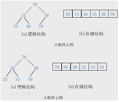
七、堆排序

1、原理方法

    BST、堆資料結構、利用陣列快速定位、無序有序區

 

2、特點

1）、穩定性：不穩定

2）、時間代價：O(n*logn)

3）、輔助儲存空間：O(1)

4）、比較

①常情況下速度要慢於快速排序（因為要重組堆）

②既能快速查詢、又能快速移動元素。

     n較大時、關鍵字元素可能出現本身是有序時適用

 3、程式碼

#include<iostream>
#include <ctime>
#include <cstring>
using namespace std;

void HeapAdjust(int array[], int i, int nLength)
{
    int nChild;
　　int nTemp;
　　
    for (nTemp = array[i]; 2 * i + 1 < nLength; i = nChild)
    {
        nChild = 2 * i + 1;

        if ( nChild < nLength-1 && array[nChild + 1] > array[nChild])
            ++nChild;

        if (nTemp < array[nChild])
        {
            array[i] = array[nChild];
            array[nChild]= nTemp;
        }
        else
            break;
    }
}

// 堆排序演算法
void HeapSort(int array[],int length)
{  
    int tmp;
    for (int i = length / 2 - 1; i >= 0; --i)
        HeapAdjust(array, i, length);

    for (int i = length - 1; i > 0; --i)
    {
        tmp = array[i];
        array[i] = array[0];
        array[0] = tmp;
        HeapAdjust(array, 0, i);
    }
}

int main()
{
    int n;
    cin >> n;
    int *data = new int[n];
    if(!data) 
        exit(1);
    int k = n;
    while(k --)
    {
         cin >> data[n-k-1];
    }

    clock_t s = clock();
    HeapSort(data, n);
    clock_t e = clock();

    k = n;
    while(k --)
    {
        cout << data[n-k-1] << ' ';
    }
    cout << endl;
    cout << "the algrothem used " << e-s << " miliseconds."<< endl;
    delete data;
    system("pause");
}

八、基數排序(桶排序)（屬於分配排序）

1、原理方法

     基數排序(radix sort）屬於分配式排序（distribution sort）、又稱桶子法（bucket sort或bin sort)。通過鍵值的查詢，將要排序的元素分配至某些“桶”中，以達到排序的作用。

1）、分配排序(hash)

①關鍵碼確定記錄在陣列中的位置，但只能對0～n-1進行排序

②(擴充套件)允許關鍵碼重複、陣列元素可變長、每個元素成為連結串列的頭節點

③(擴充套件)允許關鍵碼範圍大於n、關鍵碼值（盒子數）比記錄數大很多時效率很差(檢查是否有元素)、同時儲存的陣列變大

④(擴充套件)桶式排序、每一個盒子與一組關鍵碼相關、桶中（較少）記錄用其它方法（收尾排序）排序

⑤堆排序

2）、LSD的基數排序

適用於位數小的數列

73, 22, 93, 43, 55, 14, 28, 65, 39, 81

①首先根據個位數的數值，在走訪數值時將它們分配至編號0到9的桶子中。

0

1 81

2 22

3 73 93 43

4 14

5 55 65

6

7

8 28

9 39

②接下來將這些桶子中的數值重新串接起來，成為以下的數列。

81, 22, 73, 93, 43, 14, 55, 65, 28, 39

接著再進行一次分配，這次是根據十位數來分配：

0

1 14

2 22 28

3 39

4 43

5 55

6 65

7 73

8 81

9 93

③接下來將這些桶子中的數值重新串接起來，成為以下的數列：

14, 22, 28, 39, 43, 55, 65, 73, 81, 93

這時候整個數列已經排序完畢；如果排序的物件有三位數以上，則持續進行以上的動作直至最高位數為止。

3）、MSD

①位數多、由高位數為基底開始進行分配

②分配之後並不馬上合併回一個陣列中，而是在每個“桶子”中建立“子桶”，將每個桶子中的數值按照下一數位的值分配到“子桶”中。在進行完最低位數的分配後再合併回單一的陣列中。

 

2、特點

1)、穩定性：穩定

2）、時間代價

①n個記錄、關鍵碼長度為d(趟數)、基數r(盒子數如10)、不同關鍵碼值m(堆數<=n)

②鏈式基數排序的時間複雜度為O(d(n+r))

一趟分配時間複雜度為O(n)、一趟收集時間複雜度為O(radix)、共進行d趟分配和收集

③下面是一個近似值，可自己推導

O(nlog(r)m)、O(nlogn)（關鍵碼全不同）

m<=n、d>=log(r)m

3）、輔助儲存空間

2*r個指向佇列的輔助空間、用於靜態連結串列的n個指標

4）、比較

    ①空間允許情況下

    ②適用於：

      關鍵字在一個有限範圍內

      有些情況下效率高於其它比較性排序法

      記錄數目比關鍵碼長度大很多

      調節r得到較好效能

3、程式碼

int MaxBit(int data[],int n) 
{
    int maxBit = 1; 
    int temp =10;
    for(int i = 0;i < n; ++i)
    {
        while(data[i] >= temp)
        {
            temp *= 10;
            ++maxBit;
        }
    }
    return maxBit;
}

//基數排序
void RadixSort(int data[],int n)
{
    int maxBit = MaxBit(data,n);

    int* tmpData = new int[n];   
    int* cnt = new int[10];  
　　int  radix = 1;       
　　int  i,j,binNum;      
　　
    for(i = 1; i<= maxBit;++i) 
    {
        for(j = 0;j < 10;++j)
            cnt[j] = 0; 

        for(j = 0;j < n; ++j)
        {
            binNum = (data[j]/radix)%10; 
            cnt[binNum]++;
        }

        for(binNum=1;binNum< 10;++binNum)
            cnt[binNum] = cnt[binNum-1] + cnt[binNum]; 

        for(j = n-1;j >= 0;--j) 
        {
            binNum= (data[j]/radix)%10;            
            tmpData[cnt[binNum]-1] = data[j];    
            cnt[binNum]--;                        
        }

        for(j = 0;j < n;++j)
            data[j] = tmpData[j];
        radix = radix*10;
    }
    delete [] tmp;
    delete [] cnt;
}

轉載來自：http://m.blog.csdn.net/douyxiang/article/details/21551751