
γ = 1/scale =1/0.902
α = exp(−(Intercept)γ)=exp(-(7.111)*γ)
> library(survival)
> myfit=survreg(Surv(futime, fustat)~1 , ovarian, dist="weibull",scale=0)
> summary(myfit)

Call:
survreg(formula = Surv(futime, fustat) ~ 1, data = ovarian, dist = "weibull",
    scale = 0)
             Value Std. Error      z         p
(Intercept)  7.111      0.293 24.292 2.36e-130
Log(scale)  -0.103      0.254 -0.405  6.86e-01

Scale= 0.902

Weibull distribution
Loglik(model)= -98   Loglik(intercept only)= -98
Number of Newton-Raphson Iterations: 5
n= 26
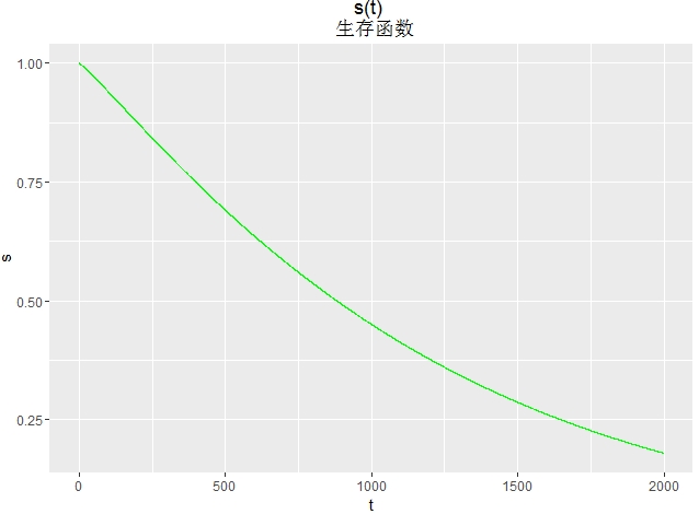
畫生存函式圖
d<- seq(0, 2000, length.out=10000)

h<-1-pweibull(d,shape=1/0.902,scale=exp(7.111))

df<-data.frame(t=d,s=h)

library(ggplot2)

ggplot(df,aes(x=t,y=s))+
  geom_line(colour="green")+
  ggtitle("s(t) \n 生存函式")
1. Surv
Description
建立一個生存物件,通常用作模型公式中的響應變數。 引數匹配是此功能的特殊功能,請參閱下面的詳細資訊。
Surv(time, time2, event,
    type=c('right', 'left', 'interval', 'counting', 'interval2', 'mstate'),
    origin=0)
is.Surv(x)
Arguments
time
對於右刪失資料,這是一個跟蹤時間。對於區間資料,第一個引數是區間的開始時間。
event
狀態指示,通常,0=活著,1=死亡。其他選擇是TRUE/FALSE (TRUE = 死亡) or 1/2 (2=死亡)。對於區間刪失資料,狀態指示,0=右刪失, 1=事件時間, 2=左刪失, 3=區間刪失.
右刪失(Right Censoring):只知道實際壽命大於某數;
左刪失(Left Censoring):只知道實際壽命小於某數;
區間刪失(Interval Censoring):只知道實際壽命在一個時間區間內。
time2
區間刪失區間的結束時間或僅對過程資料進行計數。
type
指定刪失型別。 "right", "left", "counting", "interval", "interval2" or "mstate".
如果event變數是一個因子,假定type="mstate"。如果沒有指定引數time2,type="right";如果指定引數time2,type="counting"
Surv使用示例
> str(lung)
'data.frame':	228 obs. of  10 variables:
 $ inst     : num  3 3 3 5 1 12 7 11 1 7 ...
 $ time     : num  306 455 1010 210 883 ...
 $ status   : num  2 2 1 2 2 1 2 2 2 2 ...
 $ age      : num  74 68 56 57 60 74 68 71 53 61 ...
 $ sex      : num  1 1 1 1 1 1 2 2 1 1 ...
 $ ph.ecog  : num  1 0 0 1 0 1 2 2 1 2 ...
 $ ph.karno : num  90 90 90 90 100 50 70 60 70 70 ...
 $ pat.karno: num  100 90 90 60 90 80 60 80 80 70 ...
 $ meal.cal : num  1175 1225 NA 1150 NA ...
 $ wt.loss  : num  NA 15 15 11 0 0 10 1 16 34 ...
> with(lung, Surv(time, status))
  [1]  306   455  1010+  210   883  1022+  310   361   218
 [10]  166   170   654   728    71   567   144   613   707
 [19]   61    88   301    81   624   371   394   520   574
 [28]  118   390    12   473    26   533   107    53   122
 [37]  814   965+   93   731   460   153   433   145   583
 [46]   95   303   519   643   765   735   189    53   246
 [55]  689    65     5   132   687   345   444   223   175
 [64]   60   163    65   208   821+  428   230   840+  305
 [73]   11   132   226   426   705   363    11   176   791
 [82]   95   196+  167   806+  284   641   147   740+  163
 [91]  655   239    88   245   588+   30   179   310   477
[100]  166   559+  450   364   107   177   156   529+   11
[109]  429   351    15   181   283   201   524    13   212
[118]  524   288   363   442   199   550    54   558   207
[127]   92    60   551+  543+  293   202   353   511+  267
[136]  511+  371   387   457   337   201   404+  222    62
[145]  458+  356+  353   163    31   340   229   444+  315+
[154]  182   156   329   364+  291   179   376+  384+  268
[163]  292+  142   413+  266+  194   320   181   285   301+
[172]  348   197   382+  303+  296+  180   186   145   269+
[181]  300+  284+  350   272+  292+  332+  285   259+  110
[190]  286   270    81   131   225+  269   225+  243+  279+
[199]  276+  135    79    59   240+  202+  235+  105   224+
[208]  239   237+  173+  252+  221+  185+   92+   13   222+
[217]  192+  183   211+  175+  197+  203+  116   188+  191+
[226]  105+  174+  177+


> str(heart)
'data.frame':	172 obs. of  8 variables:
 $ start     : num  0 0 0 1 0 36 0 0 0 51 ...
 $ stop      : num  50 6 1 16 36 39 18 3 51 675 ...
 $ event     : num  1 1 0 1 0 1 1 1 0 1 ...
 $ age       : num  -17.16 3.84 6.3 6.3 -7.74 ...
 $ year      : num  0.123 0.255 0.266 0.266 0.49 ...
 $ surgery   : num  0 0 0 0 0 0 0 0 0 0 ...
 $ transplant: Factor w/ 2 levels "0","1": 1 1 1 2 1 2 1 1 1 2 ...
 $ id        : num  1 2 3 3 4 4 5 6 7 7 ...
> Surv(heart$start, heart$stop, heart$event)
  [1] (  0.0,  50.0]  (  0.0,   6.0]  (  0.0,   1.0+]
  [4] (  1.0,  16.0]  (  0.0,  36.0+] ( 36.0,  39.0]
  [7] (  0.0,  18.0]  (  0.0,   3.0]  (  0.0,  51.0+]
 [10] ( 51.0, 675.0]  (  0.0,  40.0]  (  0.0,  85.0]
 [13] (  0.0,  12.0+] ( 12.0,  58.0]  (  0.0,  26.0+]
 [16] ( 26.0, 153.0]  (  0.0,   8.0]  (  0.0,  17.0+]
 [19] ( 17.0,  81.0]  (  0.0,  37.0+] ( 37.0,1387.0]
 [22] (  0.0,   1.0]  (  0.0,  28.0+] ( 28.0, 308.0]
 [25] (  0.0,  36.0]  (  0.0,  20.0+] ( 20.0,  43.0]
 [28] (  0.0,  37.0]  (  0.0,  18.0+] ( 18.0,  28.0]
 [31] (  0.0,   8.0+] (  8.0,1032.0]  (  0.0,  12.0+]
 [34] ( 12.0,  51.0]  (  0.0,   3.0+] (  3.0, 733.0]
 [37] (  0.0,  83.0+] ( 83.0, 219.0]  (  0.0,  25.0+]
 [40] ( 25.0,1800.0+] (  0.0,1401.0+] (  0.0, 263.0]
 [43] (  0.0,  71.0+] ( 71.0,  72.0]  (  0.0,  35.0]
 [46] (  0.0,  16.0+] ( 16.0, 852.0]  (  0.0,  16.0]
 [49] (  0.0,  17.0+] ( 17.0,  77.0]  (  0.0,  51.0+]
 [52] ( 51.0,1587.0+] (  0.0,  23.0+] ( 23.0,1572.0+]
 [55] (  0.0,  12.0]  (  0.0,  46.0+] ( 46.0, 100.0]
 [58] (  0.0,  19.0+] ( 19.0,  66.0]  (  0.0,   4.5+]
 [61] (  4.5,   5.0]  (  0.0,   2.0+] (  2.0,  53.0]
 [64] (  0.0,  41.0+] ( 41.0,1408.0+] (  0.0,  58.0+]
 [67] ( 58.0,1322.0+] (  0.0,   3.0]  (  0.0,   2.0]
 [70] (  0.0,  40.0]  (  0.0,   1.0+] (  1.0,  45.0]
 [73] (  0.0,   2.0+] (  2.0, 996.0]  (  0.0,  21.0+]
 [76] ( 21.0,  72.0]  (  0.0,   9.0]  (  0.0,  36.0+]
 [79] ( 36.0,1142.0+] (  0.0,  83.0+] ( 83.0, 980.0]
 [82] (  0.0,  32.0+] ( 32.0, 285.0]  (  0.0, 102.0]
 [85] (  0.0,  41.0+] ( 41.0, 188.0]  (  0.0,   3.0]
 [88] (  0.0,  10.0+] ( 10.0,  61.0]  (  0.0,  67.0+]
 [91] ( 67.0, 942.0+] (  0.0, 149.0]  (  0.0,  21.0+]
 [94] ( 21.0, 343.0]  (  0.0,  78.0+] ( 78.0, 916.0+]
 [97] (  0.0,   3.0+] (  3.0,  68.0]  (  0.0,   2.0]
[100] (  0.0,  69.0]  (  0.0,  27.0+] ( 27.0, 842.0+]
[103] (  0.0,  33.0+] ( 33.0, 584.0]  (  0.0,  12.0+]
[106] ( 12.0,  78.0]  (  0.0,  32.0]  (  0.0,  57.0+]
[109] ( 57.0, 285.0]  (  0.0,   3.0+] (  3.0,  68.0]
[112] (  0.0,  10.0+] ( 10.0, 670.0+] (  0.0,   5.0+]
[115] (  5.0,  30.0]  (  0.0,  31.0+] ( 31.0, 620.0+]
[118] (  0.0,   4.0+] (  4.0, 596.0+] (  0.0,  27.0+]
[121] ( 27.0,  90.0]  (  0.0,   5.0+] (  5.0,  17.0]
[124] (  0.0,   2.0]  (  0.0,  46.0+] ( 46.0, 545.0+]
[127] (  0.0,  21.0]  (  0.0, 210.0+] (210.0, 515.0+]
[130] (  0.0,  67.0+] ( 67.0,  96.0]  (  0.0,  26.0+]
[133] ( 26.0, 482.0+] (  0.0,   6.0+] (  6.0, 445.0+]
[136] (  0.0, 428.0+] (  0.0,  32.0+] ( 32.0,  80.0]
[139] (  0.0,  37.0+] ( 37.0, 334.0]  (  0.0,   5.0]
[142] (  0.0,   8.0+] (  8.0, 397.0+] (  0.0,  60.0+]
[145] ( 60.0, 110.0]  (  0.0,  31.0+] ( 31.0, 370.0+]
[148] (  0.0, 139.0+] (139.0, 207.0]  (  0.0, 160.0+]
[151] (160.0, 186.0]  (  0.0, 340.0]  (  0.0, 310.0+]
[154] (310.0, 340.0+] (  0.0,  28.0+] ( 28.0, 265.0+]
[157] (  0.0,   4.0+] (  4.0, 165.0]  (  0.0,   2.0+]
[160] (  2.0,  16.0]  (  0.0,  13.0+] ( 13.0, 180.0+]
[163] (  0.0,  21.0+] ( 21.0, 131.0+] (  0.0,  96.0+]
[166] ( 96.0, 109.0+] (  0.0,  21.0]  (  0.0,  38.0+]
[169] ( 38.0,  39.0+] (  0.0,  31.0+] (  0.0,  11.0+]
[172] (  0.0,   6.0]
2.survreg
擬合引數生存迴歸模型。 這些是用於時間變數的任意變換的位置尺度模型; 最常見的情況使用對數變換,建立加速失效時間模型。
survreg(formula, data, weights, subset,
na.action, dist="weibull", init=NULL, scale=0,
control,parms=NULL,model=FALSE, x=FALSE,
y=TRUE, robust=FALSE, score=FALSE, ...)
dist
y變數的假設分佈。"weibull", "exponential", "gaussian", "logistic","lognormal" and "loglogistic"。
scale
可選的固定值。如果設定<=0,scale將被估計
# survreg's scale = 1/(rweibull shape) # survreg's intercept = log(rweibull scale) # survreg結果中輸出的scale與“rweibull scale”不同
control
控制值列表,參考survreg.control()
survreg.control
survreg.control(maxiter=30, rel.tolerance=1e-09,
toler.chol=1e-10, iter.max, debug=0, outer.max=10)
maxiter
最大迭代次數
rel.tolerance
“相對容忍度”來宣告收斂
toler.chol
Tolerance to declare Cholesky decomposition singular
iter.max
與maxiter相同
debug
列印除錯資訊
outer.max
用於選擇懲罰引數的外部迭代的最大數目
convergence tolerance
/x(k+1)/=/x(k)/*Tr+Ta
其中:
k 迭代次數;
x(k+1) x的k次迭代計算值;
x(k) x的k次迭代初始值;
Tr 相對誤差
Ta絕對誤差
// 表示絕對值
因此,從上述公式我們可以得到一個重要結論:設定計算迭代誤差的時候,要全面權衡物理量的絕對值大小,同時要衡量收斂迭代值的相對誤差,這樣才能正確滿意的設定自己需要的計算誤差!
不能簡單的以為絕對誤差和相對誤差越小越好,也要杜絕tolerance設定時的隨意性(按照公式進行合理的設定是一個優秀的過程工程師的基本素質)
survreg使用示例
> library(survival)
> str(ovarian)
'data.frame':	26 obs. of  6 variables:
 $ futime  : num  59 115 156 421 431 448 464 475 477 563 ...
 $ fustat  : num  1 1 1 0 1 0 1 1 0 1 ...
 $ age     : num  72.3 74.5 66.5 53.4 50.3 ...
 $ resid.ds: num  2 2 2 2 2 1 2 2 2 1 ...
 $ rx      : num  1 1 1 2 1 1 2 2 1 2 ...
 $ ecog.ps : num  1 1 2 1 1 2 2 2 1 2 ...

> # 擬合指數模型,以下2個模型是一樣的
> survreg(Surv(futime, fustat) ~ ecog.ps + rx, ovarian, dist='weibull',
+         scale=1)
Call:
survreg(formula = Surv(futime, fustat) ~ ecog.ps + rx, data = ovarian,
    dist = "weibull", scale = 1)

Coefficients:
(Intercept)     ecog.ps          rx
  6.9618376  -0.4331347   0.5815027

Scale fixed at 1 # 注意這裡

Loglik(model)= -97.2   Loglik(intercept only)= -98
	Chisq= 1.67 on 2 degrees of freedom, p= 0.43
n= 26


> survreg(Surv(futime, fustat) ~ ecog.ps + rx, ovarian,
+         dist="exponential")
Call:
survreg(formula = Surv(futime, fustat) ~ ecog.ps + rx, data = ovarian,
    dist = "exponential")

Coefficients:
(Intercept)     ecog.ps          rx
  6.9618376  -0.4331347   0.5815027

Scale fixed at 1 # 注意這裡

Loglik(model)= -97.2   Loglik(intercept only)= -98
	Chisq= 1.67 on 2 degrees of freedom, p= 0.43
n= 26


> ##########################################
>
> str(lung)
'data.frame':	228 obs. of  10 variables:
 $ inst     : num  3 3 3 5 1 12 7 11 1 7 ...
 $ time     : num  306 455 1010 210 883 ...
 $ status   : num  2 2 1 2 2 1 2 2 2 2 ...
 $ age      : num  74 68 56 57 60 74 68 71 53 61 ...
 $ sex      : num  1 1 1 1 1 1 2 2 1 1 ...
 $ ph.ecog  : num  1 0 0 1 0 1 2 2 1 2 ...
 $ ph.karno : num  90 90 90 90 100 50 70 60 70 70 ...
 $ pat.karno: num  100 90 90 60 90 80 60 80 80 70 ...
 $ meal.cal : num  1175 1225 NA 1150 NA ...
 $ wt.loss  : num  NA 15 15 11 0 0 10 1 16 34 ...

> # weibull分佈,如果設定scale<=0,模型將使用最大似然估計,估計最優的scale
> myfit<-survreg(Surv(time, status) ~ ph.ecog + age + sex, data=lung,dist = "weibull")
> myfit
Call:
survreg(formula = Surv(time, status) ~ ph.ecog + age + sex, data = lung,
    dist = "weibull")

Coefficients:
 (Intercept)      ph.ecog          age          sex
 6.273435252 -0.339638098 -0.007475439  0.401090541

Scale= 0.731109

Loglik(model)= -1132.4   Loglik(intercept only)= -1147.4
	Chisq= 29.98 on 3 degrees of freedom, p= 1.4e-06
n=227 (1 observation deleted due to missingness)

> summary(myfit)
Call:
survreg(formula = Surv(time, status) ~ ph.ecog + age + sex, data = lung,
    dist = "weibull")
               Value Std. Error     z        p
(Intercept)  6.27344    0.45358 13.83 1.66e-43
ph.ecog     -0.33964    0.08348 -4.07 4.73e-05
age         -0.00748    0.00676 -1.11 2.69e-01
sex          0.40109    0.12373  3.24 1.19e-03
Log(scale)  -0.31319    0.06135 -5.11 3.30e-07

Scale= 0.731

Weibull distribution
Loglik(model)= -1132.4   Loglik(intercept only)= -1147.4
	Chisq= 29.98 on 3 degrees of freedom, p= 1.4e-06
Number of Newton-Raphson Iterations: 5
n=227 (1 observation deleted due to missingness)

 #   survreg's scale  =    1/(rweibull shape)
 #   survreg's intercept = log(rweibull scale)
 # survreg結果中輸出的scale與“rweibull scale”不同


##############################################
> # weibull分佈,以sex對資料分組,產生2個不同的scale
> myfit1<-survreg(Surv(time, status) ~ ph.ecog + age + strata(sex), data=lung,dist = "weibull")
> summary(myfit1)
Call:
survreg(formula = Surv(time, status) ~ ph.ecog + age + strata(sex),
    data = lung, dist = "weibull")
               Value Std. Error      z        p
(Intercept)  6.73235    0.42396 15.880 8.75e-57
ph.ecog     -0.32443    0.08649 -3.751 1.76e-04
age         -0.00581    0.00693 -0.838 4.02e-01
sex=1       -0.24408    0.07920 -3.082 2.06e-03
sex=2       -0.42345    0.10669 -3.969 7.22e-05

Scale:
sex=1 sex=2
0.783 0.655

Weibull distribution
Loglik(model)= -1137.3   Loglik(intercept only)= -1146.2
	Chisq= 17.8 on 2 degrees of freedom, p= 0.00014
Number of Newton-Raphson Iterations: 5
n=227 (1 observation deleted due to missingness)


################################################
# 具有高斯誤差的線性迴歸,以及左刪失資料
> survreg(Surv(durable, durable>0, type='left') ~ age + quant,
+         data=tobin, dist='gaussian', scale = 0)
Call:
survreg(formula = Surv(durable, durable > 0, type = "left") ~
    age + quant, data = tobin, dist = "gaussian", scale = 0)

Coefficients:
(Intercept)         age       quant
15.14486636 -0.12905928 -0.04554166

Scale= 5.57254

Loglik(model)= -28.9   Loglik(intercept only)= -29.5
	Chisq= 1.1 on 2 degrees of freedom, p= 0.58
n= 20
3.survdiff
測試在兩條或更多條生存曲線之間是否存在差異
survdiff(formula, data, subset, na.action, rho=0)
rho = 0 表示log-rank or Mantel-Haenszel檢驗;
rho = 1 表示Wilcoxon檢驗
log-rank檢驗(時序檢驗)--生存時間分佈近似weibull分佈或者屬於比例風險模型時效率較高
似然比檢驗(likelihood ratio test)--生存時間分佈近似指數分佈時效率較高
wilcoxon檢驗--生存時間分佈近似對數正態分佈效率較高
survdiff使用示例
> survdiff(Surv(futime, fustat) ~ rx,data=ovarian)
Call:
survdiff(formula = Surv(futime, fustat) ~ rx, data = ovarian)

      N Observed Expected (O-E)^2/E (O-E)^2/V
rx=1 13        7     5.23     0.596      1.06
rx=2 13        5     6.77     0.461      1.06

 Chisq= 1.1  on 1 degrees of freedom, p= 0.303


> # 用strata來控制協變數的影響
> survdiff(Surv(time, status) ~ pat.karno + strata(inst), data=lung)
Call:
survdiff(formula = Surv(time, status) ~ pat.karno + strata(inst),
    data = lung)

n=224, 4 observations deleted due to missingness.

               N Observed Expected (O-E)^2/E (O-E)^2/V
pat.karno=30   2        1    0.692   0.13720   0.15752
pat.karno=40   2        1    1.099   0.00889   0.00973
pat.karno=50   4        4    1.166   6.88314   7.45359
pat.karno=60  30       27   16.298   7.02790   9.57333
pat.karno=70  41       31   26.358   0.81742   1.14774
pat.karno=80  50       38   41.938   0.36978   0.60032
pat.karno=90  60       38   47.242   1.80800   3.23078
pat.karno=100 35       21   26.207   1.03451   1.44067

 Chisq= 21.4  on 7 degrees of freedom, p= 0.00326


> survdiff(Surv(time, status) ~ pat.karno + sex, data=lung)
Call:
survdiff(formula = Surv(time, status) ~ pat.karno + sex, data = lung)

n=225, 3 observations deleted due to missingness.

                      N Observed Expected (O-E)^2/E (O-E)^2/V
pat.karno=30, sex=1   1        1    0.246  2.31e+00  2.33e+00
pat.karno=30, sex=2   1        0    0.412  4.12e-01  4.16e-01
pat.karno=40, sex=1   1        1    0.132  5.68e+00  5.72e+00
pat.karno=40, sex=2   1        0    1.204  1.20e+00  1.22e+00
pat.karno=50, sex=1   2        2    0.111  3.23e+01  3.25e+01
pat.karno=50, sex=2   2        2    0.968  1.10e+00  1.11e+00
pat.karno=60, sex=1  18       17    9.173  6.68e+00  7.14e+00
pat.karno=60, sex=2  12       10    6.064  2.56e+00  2.68e+00
pat.karno=70, sex=1  30       23   16.737  2.34e+00  2.65e+00
pat.karno=70, sex=2  11        8    9.527  2.45e-01  2.62e-01
pat.karno=80, sex=1  32       26   24.570  8.32e-02  9.91e-02
pat.karno=80, sex=2  19       13   16.311  6.72e-01  7.55e-01
pat.karno=90, sex=1  31       25   24.992  2.66e-06  3.21e-06
pat.karno=90, sex=2  29       13   24.420  5.34e+00  6.33e+00
pat.karno=100, sex=1 21       15   14.002  7.11e-02  7.91e-02
pat.karno=100, sex=2 14        6   13.131  3.87e+00  4.25e+00

 Chisq= 66.1  on 15 degrees of freedom, p= 2.17e-08
anova
計算一個或多個擬合模型的方差(或偏差)表的分析
mod1<-survreg(Surv(time, status) ~ ph.ecog + age + sex, data=lung,dist = "weibull")
mod2<-survreg(Surv(time, status) ~ ph.ecog + age + sex+ph.karno*pat.karno, data=lung,dist = "weibull")

anova(mod1,mod2,test="Chisq")
                                       Terms Resid. Df    -2*LL Test Df Deviance     Pr(>Chi)
1                        ph.ecog + age + sex       222 2264.877      NA       NA           NA
2 ph.ecog + age + sex + ph.karno * pat.karno       215 2209.372    =  7 55.50527 1.183848e-09

library(MASS)
# 簡潔模型更好
stepAIC(mod1)
stepAIC(mod2)